
**process weibull#
Description#
This post computation provides the means for doing a Weibull analysis on a structure. Two modes of operation are available:
eigenstress\[\sigma'= \left( \frac{\sigma_1^M-\sigma_0}{\sigma_u} \right)^m\]independent\[\sigma'= \left( \frac{\sigma_1^M-\sigma_0}{\sigma_u} \right)^m + \left( \frac{\sigma_2^M-\sigma_0}{\sigma_u} \right)^m + \left( \frac{\sigma_3^M-\sigma_0}{\sigma_u} \right)^m\]
The Weibull stress is then defined as:
where \(\sigma_1^M\), \(\sigma_2^M\) and \(\sigma_3^M\) are
the post-computation results from a local fmax applied successively
to the three principal stresses \(\sigma_1\), \(\sigma_2\) and
\(\sigma_3\), in descending order. These sub-posts are run
automatically by the weibull processor.
\(V_0\), \(\sigma_u\), \(\sigma_0\) and \(m\) are material parameters:
\(m\) is the Weibull modulus. A smaller value of this parameter indicates greater dispersion, leading to a highly heterogeneous defect distribution (Fig. 12) and widely scattered failure stresses within the material volume \(V\). Conversely, a larger value reflects a more homogeneous defect distribution (Fig. 13), resulting in lower variability of failure stresses within the same volume.
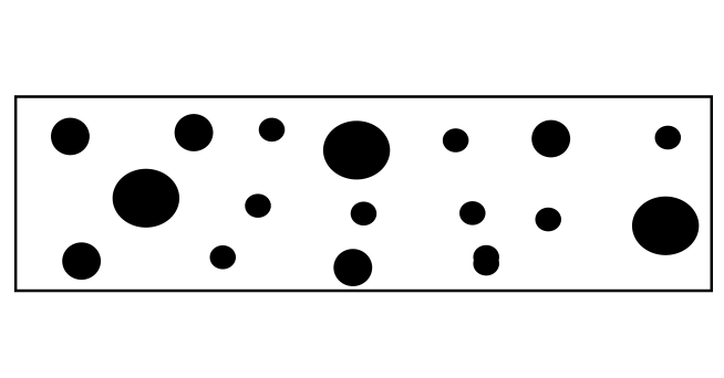
Fig. 12 Defect distribution in a material with a low Weibull modulus.#
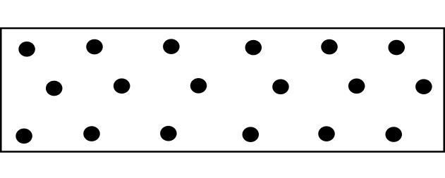
Fig. 13 Defect distribution in a material with a high Weibull modulus.#
\(V_0\) is the reference (elementary) volume. A specimen of volume \(V\) is considered to be composed of an assembly of elementary volumes \(V_0\). The probability of failure of a specimen of volume \(V\) is therefore related to the probability of failure of a specimen of volume \(V_0\).
To better illustrate this:
Consider a specimen of volume \(V_0\) subjected to a given load. Let its probability of failure be \(P_{F0}\), and its probability of survival be \(1-P_{F0}\).
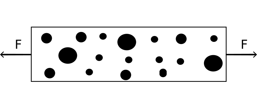
Fig. 14 Tensile tests on a specimen of volume \(V_0\).#
Now, imagine a series system composed of two identical specimens of volume \(V_0\), all subjected to the same stress. The probability of survival of this system is:
\[P(1 \cap 2) = (1-P_{F0})^2 \Rightarrow \log((1-P_{F0})^2)= 2 \log(1-P_{F0})\]
Fig. 15 Tensile tests on a specimen of volume \(2\times V_0\).#
Therefore, the probability of survival of a specimen with a length \(n\) times greater (and thus a volume \(n\) times larger than \(V_0\)) is:
\[\log(1-P_{FN})=n\log(1-P_{F0})\]Hence, the probability of survival of a specimen of volume \(V\) is related to that of the reference volume \(V_0\) by:
\[\log(1-P_{FN})= \frac{V}{V_0} \log(1-P_{F0})\]
The probability of failure \(P_r\) is then given by:
In addition to the output of \(\sigma_W\) and \(P_r\). The
values of \(\sigma'\) are stored at each Gauss point under a name
constructed by adding _wb to the variable name.
Syntax#
**process weibull
\(~\,\) *var name
\(~\,\) *mode eigenstress | independant
\(~\,\) *coefmin value1
\(~\,\) *coefmax value2
\(~\,\) *file namef
*varnamename of stress variable.
If the user has only specified a single map (with output_number),
the history is reconstructed from the values read after the options
*coefmin and *coefmax. \(\sigma_1^M\) varies linearly over
100 maps of value1 \(\times \sigma_1\) to
value2 \(\times \sigma_1\) (where \(\sigma_1\) is calculated at
the specified map).
With the option *file, the history is read in the file namef, of
the form:
0.01     10
0.02     15
0.03     20
0.04     40
0.05     60
...
where the first column represents the time and the second the value of \(\sigma_1\).
These two methods presented for the mode eigenstress extend to the
mode independent as well.
Example#
****post_processing
 ***global_post_processing
  **output_number 10
  **process weibull
   *var sig
   *mode independent
   *coefmin 0.5
   *coefmax 2.5
****return

   % material file
  ***post_processing_data
   **process weibull
     V0      10.
     m       20.
     sigma_u 1200.
     sigma_0 0.
  ***return