ISOTROPIC#
Description#
This object class defines models of isotropic hardening for use in a variety of material behaviors and potentials. Isotropic hardening causes an isotropic expansion or contraction of the yield surface in stress tensor space. The isotropic hardening may be a function of the simulated multiplier which is normally equal to the cumulative plastic strain equivalent \(p\), or in terms of its own internal variable. The latter must be used for cases of static recovery.
The initial value \(R_0\) for the yield radius is noted here to be the onset of plasticity, and not the engineering yield stress. It may thus be found to be significantly lower than expected.
Syntax#
The syntax to specify a isotropic hardening object will consist of giving the keyword for a particular law desired, followed by a list of appropriate coefficients which are dependent on the model chosen. The possible isotropic laws are the following:
CODE |
DESCRIPTION |
|---|---|
|
initial value only (perfect plasticity). |
|
(or |
|
linear hardening followed by perfect plasticity. |
|
power law of \(p\). |
|
hardening defined by a list of experimental points in an external datafile. |
|
another hardening defined by a table of points. For a series of temperatures, different stress strain curves to be entered. |
|
nonlinear, exponentially saturating function of \(p\). |
|
nonlinear with kinematic interaction (for use with the |
|
combined linear and nonlinear saturating hardening. |
|
multiple term nonlinear hardening. |
|
multiple term nonlinear hardening. This law is rigorously equal to
|
|
hardening according to a user-defined function of \(p\). |
|
yield stress defined as the sum of several isotropic objects (see isotropic_sum). |
|
hardening function including dynamic strain aging (see isotropic_dsa). |
|
see isotropic_dsa_p. |
|
see isotropic_dsa_r. |
Only the laws with an internal variable may have static recovery and be
used in state interactions. Isotropic hardening is available with
positive values of the Q or H parameters (depending on the
model), while softening occurs with negative values of these
coefficients. The saturation rate coefficients b are necessarily
positive. All parameters may have the normal dependencies through the
COEFFICIENT mechanism.
constantThis gives the radius as a single coefficient
R0.
linear(or
iso_linear) Law with initial radius and a linear evolution depending on the cumulative inelastic strain \(p\) (i.e. \(R={\tt R0} + {\tt H}p\)) and using the coefficientsR0andH.
linear_pplinear hardening with an initial radius
R0and slopeHup toRu(i.e. \(R={\tt R0} + {\tt H}p\) for \(R<{\tt Ru}\)), followed by perfect plasticity at \(R={\tt Ru}\).

power_lawGives a power-law evolution according to
\[R = R_0 + K \left( e_0 + p \right) ^{n}\]with the coefficients
R0,K,e0,n, and \(p\) the cumulative inelastic strain. Negative values fore0are set to zero. The case \(n<1\) with \(e_0=0\) gives an infinite derivative at the onset of inelastic deformation and is therefore not allowed. Use a very small value fore0instead.
nonlinearThis law gives a nonlinear saturating evolution:
\[R = {\tt R0} + {\tt Q}\left(1 - e^{-{\tt b}p}\right)\]where the saturation radius will be \({\tt R0}+{\tt Q}\) for large \(p\). The law will reach \(95\%\) of the saturation value at \(p\approx 3.0/{\tt b}\) so that higher values of
bgive a more rapid saturation.
linear_nonlinearlinear hardening with an initial radius
R0followed by a combined linear and nonlinear evolution with coefficientsH,Qandb, according to\[R = {\tt R0} + {\tt H}p + {\tt Q}\left(1-e^{-{\tt b}p}\right).\]
nonlinear_sumThis law allows fine tuning of the isotropic hardening by use of multiple-term evolution. For instance, two terms might be combined analogous to short and long term mechanisms. There is no upper limit for the number of terms
N. The radius is calculated as:\[R = R_0 + \sum_{i}^{N} Q_i \left(1 - e^{-b_i p}\right)\]with coefficients
R0,Q1,Q2,...,QN, andb1,b2,...,bN.
-
1For Z-mat versions 9.1.5 and earlier, this model is referred to as
nonlinear_static_recovery1For Z-mat versions 9.1.5 and earlier, this model is referred to asnonlinear_v2.The hardening function is defined in terms of an integrated variable
r, whose evolution equation is governed by:\[\dot{r}=\dot{\lambda}~{\tt alpha}\left(1-\dfrac{\left<R-{\tt R0}\right>}{\tt Q}\right)-\left(\dfrac{\left<R-{\tt R0}-{\tt Rpp}\right>}{\tt M}\right)^{\tt m}\]The material coefficients are
R0,alpha,b,Q,Rp,Rpp,m, andM. By defaultalpha\(=1\). The isotropic hardening function is given by \(R={\tt R0}+{\tt b Q}r\).Note
When the value of \(\tt M\) is exteremely large (and \({\tt alpha} = 1\)), this model is equivalent to
nonlinear. In this case, we integrate \(\dot{r}=\dot{\lambda}\left(1-{\tt b} r\right)\), obtaining\[r=\dfrac{1-e^{-bp}}{b}\]The hardening function is \(R={\tt R0}+{\tt Q b}r={\tt R0}+{\tt Q}(1-e^{-{\tt b}p})\).
The evolution of \(r\) is influenced by two competing effects: hardening and recovery. The recovery term is always active, and when it is dominant (due to lower values of \({\tt M}\), or higher values of \(\tt p\)) it can suppress the hardening term.
nonlinear_v2.Iostropic hardening function defined as a list of points
The list of points describing the evolution of equivalent yield stress in terms of cumulative plastic strain can be specified in various ways:
by_pointGives the isotropic curve as input by a list of points (see the example). The first column should be
sigeqand the second is the cumulative plastic strain. Linear interpolation is performed between the given data points. When the current value of \(p\) exceeds the last value specified in the data, the isotropic hardening no longer changes, as if the isotropic hardening saturates.
*isotropic by_point\(~\,\)sigeqepcum[ parameter ] \(~\,\) s1 p1 [ val1 ] \(~\,\) s2 p2 [ val2 ] \(~\,\) … \(~\,\) sN pN [ valN ]where si: yield stress value, pi: cumulative plastic strain, and vali: parameter value.
table2Gives the isotropic curve as input by a list of points for each value of the external parameter
*isotropic table2\(~\,\) parameter val1 \(~\,~\,\) p11 s11 \(~\,~\,\) … \(~\,~\,\) p1m s1m \(~\,\) parameter val2 \(~\,~\,\) p21 s21 \(~\,~\,\) … \(~\,~\,\) p2m s2m \(~\,\) … \(~\,\) parameter valN \(~\,~\,\) pN1 sN1 \(~\,~\,\) … \(~\,~\,\) pNm sNm
where sij: yield stress value, pij: cumulative plastic strain, and vali: parameter value.
Examples#
An example of a three-term nonlinear hardening with a very rapid initial hardening, a very slow hardening (third term) and an intermediate softening (negative
Q2). Note: these are not necessarily reasonable values.*isotropic nonlinear_sum R0 50. Q1 30. b1 2000. Q2 -10. b2 20. Q3 40. b3 2.
The next example shows the use of
*isotropic by_point.**potential gen_evp ep *criterion mises *flow plasticity *isotropic by_point sigeq epcum 130.0 0.0000 140.0 0.0001 145.0 0.0002 150.0 0.0004 160.0 0.0009 170.0 0.0017 180.0 0.0028
The following gives a point-by-point specification of an isotropic hardening for an anisothermal case. Between two data points, interpolation is linear (as with all Z-set tables). For \(p>0.1\) it uses the values of 0.1 because that was the last specified. Two alternative data inputs are possible, using*isotropic by_pointor*isotropic table2syntax.The examples are provided below :*isotropic by_point sigeq epcum temperature 220. 0.0 1000. 200. 0.0 1200. 230. 0.1 1000. 210. 0.1 1200.
*isotropic table2
 temperature 1000.
  0.0 220.
  0.1 230.
 temperature 1200.
  0.0 180.
  0.1 190.
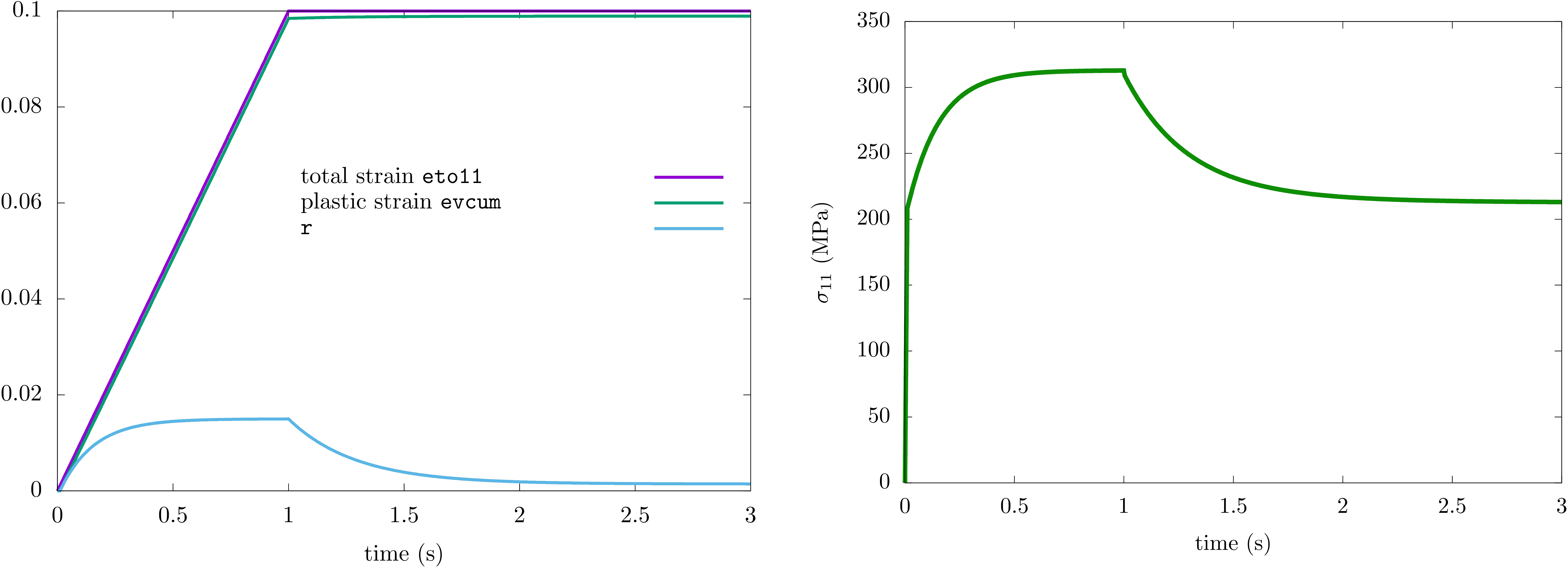
Consider the following relaxation test: a tensile load is applied with a strain that increases linearly from \(t=0\) to \(t=1\). Upon reaching a strain of \(0.1\) at \(t=1\), it remains constant until \(t=3\).
Beyond \(t=1\), the variation of plastic strain is small due to the small elastic strain, as the total strain rate satisfies \(\dot{\varepsilon}=\dot{\varepsilon}^e+\dot{\varepsilon}^p =0\). Hence, the evolution equation for the variable \(r\) becomes
\[\dot{r} \approx -\left(\dfrac{\left<R-{\tt Rpp}\right>}{{\tt M}}\right)^{\tt m}\]The recovery rate follows an exponential trend, increasing with larger values of the power \(\tt m\) or lower values of \(\tt M\).
***behavior gen_evp
 **elasticity isotropic
   young 200000.
   poisson 0.300000
 **potential gen_evp ev
  *criterion mises
  *flow norton
   n 10.0000
   K 10.0000
  *isotropic nonlinear_static_recovery
   R0 200.000
   Q 200.000
   b 35.
   Rpp 10.0000
   M 2000.00
   m 1.00000
  ***return