
Hertz contact#
Highlights
Create the mesh of the quarter of two disks using axisymmetric elements.
Comparison of finite element solutions for contact pressure and displacement.
Problem specification#
The problem involves analyzing the contact mechanics between two elastic spheres S1 and S2, with radii \(R_1\) and \(R_2\), respectively, when subjected to a compressive load \(F\).
Key Parameters:
Radii of the spheres: \(R_1=0.5\) mm and \(R_2=1\) mm.
Young’s Moduli: \(E_1=69000\) MPa and \(E_2=82000\) MPa.
Poisson’s ratios: \(\nu_1=0.33\) and \(\nu_2=0.206\).
Applied normal load: \(F=200 N\).
Assumptions:
Both spheres are isotropic and elastic.
Deformations are small relative to the radii of the spheres.
Contact is frictionless.
An axisymmetric finite element model will be used for the simulation.
Analytical solution#
The analytical solution to this problem is widely available in numerous classical references on contact mechanics (e.g. [T7]).
The contact pressure is given by \(p(r)=p_0\sqrt{1-(\dfrac{r}{a})^2}\) with \(p_0=\dfrac{3F}{2\pi a^2}\).
The radius of the contact circle is \(a=\dfrac{\pi p_0 R}{2E^\star}\).
The mutual displacement of distant points \(\delta=\dfrac{a^2}{R}\)
where \(\dfrac{1}{E^\star}=\dfrac{1-\nu_1^2}{E_1}+\dfrac{1-\nu_2^2}{E_2}\) and \(\dfrac{1}{R}=\dfrac{1}{R_1}+\dfrac{1}{R_2}\).
Mesh generation#

Fig. 81 The geometry of two semicircular disks.#
Open Zmaster GUI
Click on

Create points

#Points   x       y       z

point0    0.      0.      0.
point2    1.      0.      0.
point1    0.5     0.      0.
point3    0.      0.5     0.
point5    0.425   0.425   0.
point4    0.      1.      0.
point6    0.      1.5     0.
point7    0.      2.      0.
point8    0.5     2.      0.
point9    0.25    2.      0.
point10   0.      1.75    0.
point11   0.21    1.79    0.
Create lines

Select 2 Points or Segments w/points \(\longrightarrow\) Go.
Create lines (see Fig. 82)
Create arcs

Select Arc: center, pt1, pt2 \(\longrightarrow\) Go.
For each arc, click on the center first, followed by the two endpoints of the arc in a counterclockwise direction.
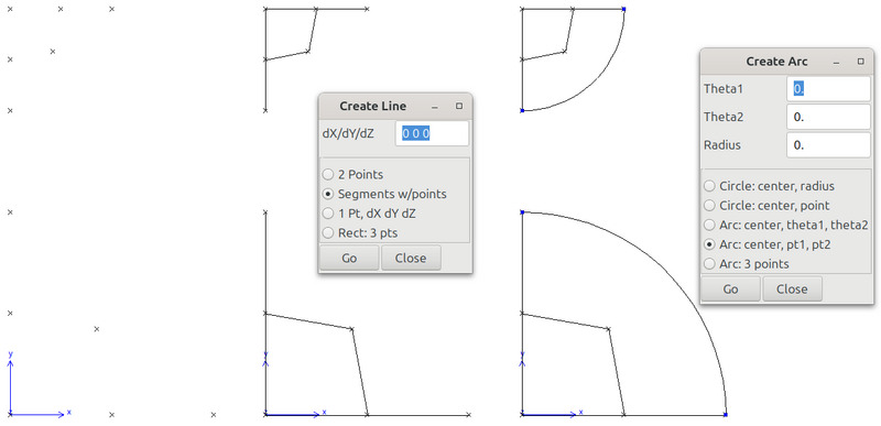
Fig. 82 Create points, lines and arcs.#
Subdivide arcs at their midpoint.
create a line between the center of top (resp. bottom) disk and the point at \((0.21,1.79)\) (resp. \((0.425, 0.425)\)).
click on
 , set R to 0, select Divide both \(\longrightarrow\) Go.
select the created line and the previously created arc. This will create the intersection point between the line and the arc.
Remove the excess line: select the line \(\longrightarrow\) Edit \(\longrightarrow\) Delete.
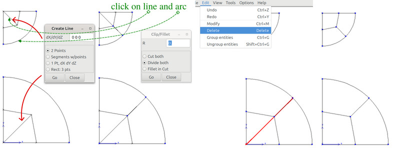
Note
This method is best suited for complex geometries where finding the intersection between two curves is challenging. However, it may not be the most efficient choice for simpler cases. For instance, in the case of the bottom disk, before creating the arc, you can directly place a point at the coordinates \((\sqrt{2}/2, \sqrt{2}/2)\). Then, connect this point to \((0.425, 0.425)\) with a line and ultimately create two arcs.
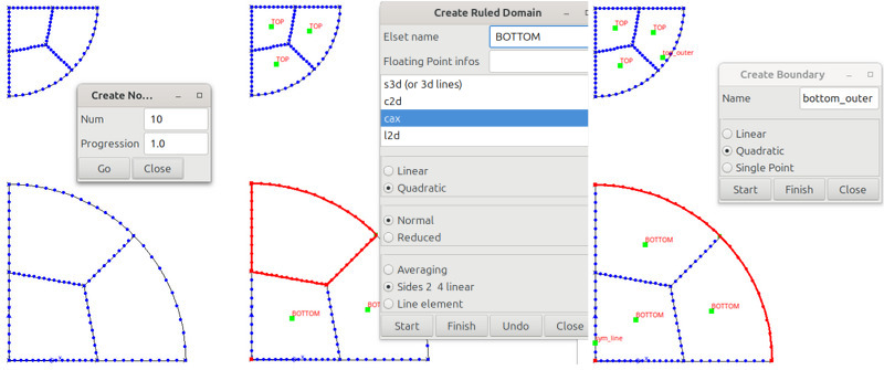
Specify the number of nodes at each edge
 .
.Create Ruled domains

Specify the Elset name, select cax, quadratic, Normal, and Sides 2 4 linear.
Click on Start, and then select the boundaries of each domain (the second and fourth sides should be lines) \(\longrightarrow\) Finish.
This will create elements of type
cax8(quadratic axisymmetric elements with full integration).Define boundary sets on which boundary conditions will be applied later

liset
sym_line: vertical lines with x=0.liset
bottom_outer: the arc segments of the bottom disk.liset
top_outer: the arc segments of the top disk.liset
bbottom: the horizontal line segments with y=0.liset
ttop: the horizontal line segments with y=2.
For each liset, choose Quadratic \(\longrightarrow\) Start, then select the curves that form the boundary set \(\longrightarrow\) Finish.
For the contact, ensure that the normals to the boundary sets (
bottom_outerandtop_outer) are oriented outward. To verify and adjust this:Click on
 .
.Scroll through the list of “meshers” until you find
bset_align.Select it and click New.
Specify the list of bsets whose normals need adjustment. To realign all normals, set bsets (list) to
ALL\(\longrightarrow\) OK.
Apply a translation of the upper part (S1),
Click on
.Scroll through the list of “meshers” until you find
translate.Select it and click New.
Set the value of y to -0.5 and elset_name to
TOP\(\longrightarrow\) OK.
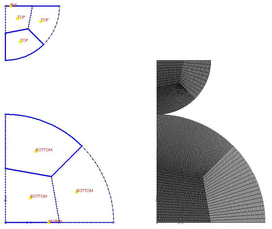
Mesh the domains

Visualize the mesh

Finite element analysis#
Finite element formulation#
A small strain axisymmetric finite element model is used for this simulation.
****calcul
 ***mesh          % 3D small_deformation by default
  **file two_disks.geof
Global problem resolution#
A Newton algorithm is used to solve the global problem. The loading sequence is applied from time=0 to 1:
the number of increments is 5,
the number of allowed iterations per increment is set to 10,
ratio of convergence is 0.01% (Residual/F_ext< 1e-4),
the tangent matrix is updated at each iteration (
p1p2p3algorithm),automatic time stepping is used to allow us to start with a small first \(\Delta t\) and then increase it as the simulation converges after each increment (until it reaches the time step given by time_sequence/increment=1/2=0.5),
**init_d_dof: to accelerate convergence, the last converged solution \(\Delta DOF\) for the last increment is used as an initial guess for the next increment.
***resolution   % by default newton
 **sequence
  *time  1.
  *increment 2
  *iteration 10
  *ratio automatic 0.01
  *algorithm p1p2p3
 **automatic_time
  *security 1.2
  *divergence 2. 10
  *first_dtime 1. 1e-3
 **init_d_dof
Boundary conditions#
The displacement of node set
sym_linein the x-direction is set to 0.The displacement of node set
bbottomin the y-direction is set to 0.A pressure is applied on the boundary set
ttop. The value of pressure is computed as \(P =F/S=F/(\pi R_1^2)\), since the model is axisymmetric. Note that the imposed value is negative because the loading direction opposes the surface normal defined by the bsetttop.
***bc
 **impose_nodal_dof
   sym_line U1 0.
   bbottom U2 0.
 **pressure
   ttop -127.324 time
Contact definition#
A contact zone is defined between the outer surfaces of both spheres
bottom_outerandtop_outer.*warning_distance: to define the critical distance between a slave node and the closest point on the master surface, below which a contact element is created.*clearance: to adjust the contact between surfaces (remove any gap or penetration in the initial mesh). Only nodes of the slave surface that are within the clearance distance in the initial geometry are moved onto the master surface (see adjust contact).
***continuum_contact
 **zone penalty
  *master bottom_outer
  *slave top_outer
  *warning_distance 1.
  *clearance -1e-12
Material behavior#
The material behavior for TOP and BOTTOM elsets is specified. If the material behavior is
defined in the same input file, use *this_file command and then specify the number of the material
behavior by definition order withing the file. Since the material behavior is elastic, no integration
method for constitutive equations is required.
***material
 **elset TOP
  *this_file 1
 **elset BOTTOM
  *this_file 2
****return

***behavior gen_evp
 **elasticity  isotropic
   young 69000.
   poisson 0.33
***return

***behavior gen_evp
 **elasticity  isotropic
   young 82000.
   poisson 0.206
***return
Results & discussions#
To visualize results:
Launch the command
Zmaster contact_two_disks
Click on
 , and select variables on nodes or integration points to visualize.

Fig. 83 The finite element results: (a) the displacement U2 (b) the stress sig22 (c) sig11
(d) sig12 (e) von Mises stress.#
Analytical |
finite element |
|---|---|
\(p_0 = 6603.653\) |
\(\approx 6642\) |
\(\delta =0.02169\) |
\(\approx 0.02153\) |
\(a =0.085\) |
\(\approx 0.0849\) |
To plot the value of pressure across the contact area:
Click on

Select liset: bottom_outer, and select x vs. sig22 \(\longrightarrow\) Draw.
To plot only within the contact region, adjust the X-range by clicking on More …, setting Xmin and Xmax values, and unchecking Auto X range \(\longrightarrow\) Apply.
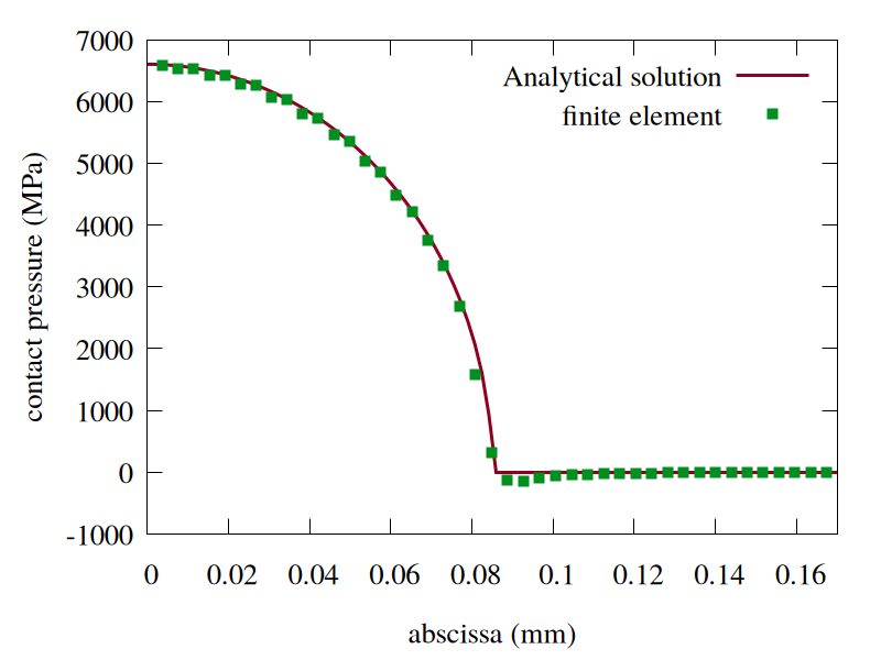
Fig. 84 Comparison of contact pressure results from finite element analysis and analytical solution.#
Downloads
Mesh files
Input files