A elastoplastic analysis of a disk under rotation

Highlights

This tutorial explores the following topics:

• Mesh a simple geometry.

• Apply a centrifugal force.

• Estimate the limit rotational speeds of bored disks.

• Compare results of a ‘thin’ and a ‘thick’ disk.

Problem specification

Rotating machines are common in industrial structures. Discs and shafts are critical parts in, for example, aircraft engines and turbines for power generation. They are subject to high centrifugal forces and must not fail. Therefore, their design is crucial for the integrity of the structure in service.

The objective of this tutorial is to estimate the limit rotational speeds of bored disks. We assume that material model of the disk is perfectly elasto-plastic. In this problem, we consider isothermal conditions under small perturbations. The rotational speed of the disk burst can be estimated by the speed that leads to the propagation of plasticity throughout the disk.

Two cases are considered: the case of a thin disk and the case of a thick disk. In the first case, plane stress conditions are applied. The analytical solutions are detailed in [T3, T4]. In the second case, this hypothesis is not satisfied anymore. Some finite element results for that case are provided. In the rotating frame of reference attached to the disk, the equilibrium equations are given by

\[\text{div} \ten{\sigma}+\rho\vect{f}=0\]

where \(\rho\) is the material density and \(\rho \vect{f} = \rho \omega^2 r \vect{e}_r\) is the volume forces induced by the angular velocity \(\omega\).

Analytical solutions

The analytical solution of a simplified version of this problem is given in [T4] for an axisymmetric thin disk under plane stress conditions. In the latter reference, solutions are given for a Tresca plasticity criterion. The analytical solution for von Mises is inextricable since the stress components \(\sigma_{rr}\) and \(\sigma_{\theta\theta}\) are coupled.

Summary of analytical solutions for Tresca plasticity model:

• Radial stress \(\sigma_{rr}\)

\[ \begin{align}\begin{aligned}\sigma_{rr}^p &= \sigma_0 \left(1-\dfrac{r_i}{r}\right)-\dfrac{\rho\omega^2r^2}{3}\left(1-\left(\dfrac{r_i}{r}\right)^3\right) & , \quad r_i\leq r \leq a\\\sigma_{rr}^e &= -\dfrac{\rho\omega^2r^2}{8}\left(3+\nu\right) + \dfrac{A}{r^2}+B & , \quad a\leq r \leq r_e\end{aligned}\end{align} \]

where a is the location of the elastic-plastic boundary. It can be computed by solving \(\sigma_{\theta\theta}(r=a)=\sigma_0\).

• Tangential stress \(\sigma_{\theta \theta}\)

\[ \begin{align}\begin{aligned}\sigma_{\theta \theta}^p &= \sigma_0 \qquad, \quad &r_i\leq r \leq a\\\sigma_{\theta \theta}^e &= -\dfrac{\rho\omega^2r^2}{8}\left(1+3\nu\right) - \dfrac{A}{r^2}+B \qquad, \quad &a\leq r \leq r_e\end{aligned}\end{align} \]

• Radial strain \(\varepsilon_{rr}\)

\[ \begin{align}\begin{aligned}\varepsilon_{rr}^p &= 0 & , \quad r_i\leq r \leq a\\\varepsilon_{rr}^e &= \dfrac{\rho\omega^2r^2}{8E}\left(3(\nu^2-1)+(3+\nu)\left((1-\nu)\dfrac{r_i^2+r_e^2}{r^2}-(1+\nu)\dfrac{r_i^2r_e^2}{r^4}\right)\right) & , \quad a\leq r \leq r_e\end{aligned}\end{align} \]

• Tangential strain \(\varepsilon_{\theta \theta}\)

\[ \begin{align}\begin{aligned} \varepsilon_{\theta \theta}^p &= \dfrac{1}{E}\left(\dfrac{r_i}{r}\log{\dfrac{r}{a}}\left(\dfrac{\rho\omega^2r_i^2}{3}-\sigma_0\right)-\dfrac{\rho\omega^2r^2}{9}(1+3\nu)\left(1-\left(\dfrac{a}{r}\right)^3\right)\right) &, \quad r_i\leq r \leq a\\\varepsilon_{\theta \theta}^e &= \dfrac{\sigma_{\theta \theta}^e}{E}-\nu\dfrac{\sigma_{rr}^e}{E} & , \quad a\leq r \leq r_e\end{aligned}\end{align} \]

• Radial displacement \(u_r\)

\[ \begin{align}\begin{aligned} u_r^p &= \dfrac{1-\nu}{E}\sigma_0 r - \dfrac{\sigma_0r_i}{E}\log{\dfrac{r}{r_e}}-\dfrac{\rho\omega^2}{3E}\left(\dfrac{r^3}{3}-r_i^3\log{\dfrac{r}{r_e}}\right) + \dfrac{C}{E} & , \quad r_i\leq r \leq a\\u_r^e &= \dfrac{1}{E}\left(\dfrac{\rho\omega^2r^3}{8}(\nu^2-1)-\dfrac{A}{r}(1+\nu)+Br(1-\nu)\right) & , \quad a\leq r \leq r_e\end{aligned}\end{align} \]

where \(A\), \(B\) and \(C\) are integration constants given by

\[ \begin{align}\begin{aligned}A &= -\dfrac{\sigma_0}{2}ar_i + \dfrac{\rho\omega^2a^4}{6}\left(-\dfrac{1+3\nu}{4}+\left(\dfrac{r_i}{a}^3\right)\right)\\B &= \sigma_0\left(1-\dfrac{r_i}{2a}\right) + \dfrac{\rho\omega^2a^2}{6}\left(\dfrac{1+3\nu}{2}+\left(\dfrac{r_i}{a}^3\right)\right)\\C &= -r_i\left(\log{\dfrac{a}{r_e}}+\nu\right)\left(\dfrac{\rho\omega^2r_i^2}{3}-\sigma_0\right) + \dfrac{\rho\omega^2a^3}{9}(1+3\nu)\end{aligned}\end{align} \]

Mesh generation

Fig. 50 A schematic representation of a bored turbine disk. The cylindrical coordinates are adopted. For 2D case, simulations are considered in the x-y plane which means that the rotation axis is parallel to \(\vect{e}_y\).

• Create points

  • for a thin disk:

  #Points  x    y    z
  
  point0   5.   0.   0.
  point1   50.  0.   0.
  point2   50.  0.1  0.
  point3   5.   0.1  0.
  

  • for a thick disk:

  #Points  x    y    z
  
  point0   5.   0.   0.
  point1   50.  0.   0.
  point2   50.  10.  0.
  point3   5.   10.  0.
  

• Create lines

• Specify the number of nodes at each edge

• Create a ruled domain

  

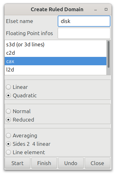
  Fig. 51 The disk is meshed using axisymmetric elements cax8r (quadratic elements with reduced integration).

• Create boundary sets (see Fig. 52)

• Mesh the domain

Fig. 52 The mesh of a thick disk and the boundary sets .

The user can also download the geometry file disk_thin.mast. Open the file with Zmaster and mesh the domain by clicking on \(\longrightarrow\) (or run the command Zrun -B thin_disk.mast). The position of points in the .mast file can be modified to change the disk dimensions.

Finite element analysis

Finite element formulation

A small strain axi-symmetric model is used for this simulation.

****calcul
 ***mesh                % by default 3D small_deformation
  **file disk_thin.geof

Global problem resolution

To solve the global problem, a Newton-Raphson algorithm is used.

• One loading sequence from time = 0 to time = 1: the number of increments is set to 20, with a maximum number of iterations of 10. The relative convergence ratio is \(0.1\%\). The tangent matrix will be updated at each iteration (*algorithm p1p2p3).

• Automatic time-stepping: the first increment \(\Delta t\) is 0.01. If the algorithm converge, the time-step will be multiplied by \(1.2\) (*security) and if it diverges the time-step will be divided by 2 with a maximum number of divergence 10. The option global 6 is used to subdivide time-step for the subsequent increment if the number of iterations per increment exceeds 6.

***resolution  % by default newton
 **sequence 1
  *time 1.
  *increment 20
  *iteration 10
  *ratio 0.1
  *algorithm p1p2p3
 **automatic_time global 6
   *security  1.2
   *divergence  2. 10
   *first_dtime 0.01

Boundary conditions

We consider a symmetric disk w.r.t to the plane defined by \(z=0\) (or \(y=0\) in the simulation) which corresponds to the boundary set bottom. The displacement of the inner part of the disk (hub) in the radial direction is set to zero. The disk rotates at a constant angular velocity \(\omega \vect{e}_z\).

***bc
 **impose_nodal_dof
   bottom U2 0.
   hub U1 0.
 **centrifugal
   ALL_ELEMENT (0.0 0.0) d2 10000. time % omega = 10000 rad/s

Material behavior

We consider a perfect elastoplastic material model with Young modulus \(E=205000\) MPa and a Poisson’s ratio of \(\nu=0.3\). Two plasticity criteria are adopted: von Mises and Tresca.

% elastoplastic.mat
***behavior gen_evp
 **elasticity isotropic
   young 205000.
   poisson 0.3
 **potential gen_evp ep
  *criterion tresca % or mises
  *isotropic constant
   R0 1000.
***coefficient
  masvol 8.08e-9
***return

Note

In Z-set, the implemented version of the Tresca model is slightly different than the standard version found in literature since the normal to the yield surface of Tresca model at the corners is chosen as the average of intersecting surfaces normals. Alternatively, one can consider the Hosford model given by

\[\sigma_{eq}=\left[\dfrac{(\sigma_I-\sigma_{II})^a+(\sigma_{II}-\sigma_{III})^a+(\sigma_{I}-\sigma_{III})^a}{2}\right]^{1/a}\]

where \(\sigma_I\), \(\sigma_{II}\), and \(\sigma_{III}\) are principal stresses. The Hosford model becomes equivalent to Tresca one by choosing higher values of the parameter \(a\).

To integrate constitutive equations, an implicit generalized midpoint integration method (theta_method_a) is used, with \(\theta=1\), a tolerance of \(10^{-12}\), and the maximum number of iterations is set to \(100\).

***material
  *file elastoplastic.mat
  *integration theta_method_a 1. 1e-12 100

Results & discussion

Thin disk

Comparison between Tresca and von Mises plasticity criteria

Fig. 53 Analytical (lines) and numerical (marked points) solutions for a Tresca perfect plasticity model. \(r_i=5 mm\) and \(r_e=50 mm\) (thickness \(H=1 mm\))

Fig. 54 Finite element solution for a von Mises perfect plasticity model. \(r_i=5 mm\) and \(r_e=50 mm\) (thickness \(H=1 mm\))

Thick disk

Consider a thick disk, with its thickness H being significant in comparison to its external radius \(r_e\) (\(H/r_e=0.2\)). The finite element solutions are provided for both Tresca and von Mises perfect plasticity models. When the disk is not “thin” anymore, the stress components \(\sigma_{zz}\) and \(\sigma_{rz}\) do not vanish. Moreover, the fields of \(\sigma_{zz}\) and \(\sigma_{rz}\) are dependent on the z-coordinate. The stress components \(\sigma_{rr}\) and \(\sigma_{\theta\theta}\) exhibit a slight variation along \(z\) (or \(y\) in figures above), which will become more pronounced when the thickness of the disk is increased.

Fig. 55 Stress fields \(\sigma_{rr}\), \(\sigma_{\theta\theta}\), \(\sigma_{zz}\), and \(\sigma_{rz}\) obtained by the finite element method for a thick disk. Results are obtained for a Tresca perfect plasticity model. Displacements have been exaggerated for illustration purposes (\(\times 100\)). The initial state of the disk is shown in red.

Fig. 56 Stress fields \(\sigma_{rr}\), \(\sigma_{\theta\theta}\), \(\sigma_{zz}\), and \(\sigma_{rz}\) obtained by the finite element method for a thick disk. Results are obtained for a von Mises perfect plasticity model.

Downloads

• Mesh files

  disk_thin.mast

  disk_thick.mast

• Input files

  disk_thick_rotation_tresca.inp

• Miscellaneous

  plot_analyt.gnu