
Perforated plate#
Highlights
This tutorial explores the following topics:
Mesh of a perforated plate with elliptical holes using Zmaster GUI, or using an ad-hoc mesher.
Compute stress and strain values expressed in cylindrical coordinate systems.
Compute the gradient of stress/strain along a line set.
Problem specification#
In this tutorial, we will explore the problem of a plate with an elliptic hole subjected to uniform tensile stress. The finite element results will be compared to analytical solutions where available. First, we will start with a circular hole subjected to a uniform uni-axial tensile stress. Then we will discuss the effect of larger holes compared to the plate dimensions. Finally, we will consider elliptic holes.
Analytical solutions#
Plate with a circular hole subjected to a uniform uni-axial tensile stress:

The stress field solution as found by Kirsch [T2] in cylindrical coordinates is given by
\[\begin{split}\begin{aligned} \sigma_{rr}(r,\theta)&=\dfrac{\sigma_\infty}{2}\left(1-\dfrac{a^2}{r^2}\right)+\dfrac{\sigma_\infty}{2}\left(1+\dfrac{3a^4}{r^4}-\dfrac{4a^2}{r^2}\right)\cos{(2\theta)}\\ \sigma_{\theta\theta}(r,\theta)&=\dfrac{\sigma_\infty}{2}\left(1+\dfrac{a^2}{r^2}\right)-\dfrac{\sigma_\infty}{2}\left(1+\dfrac{3a^4}{r^4}\right)\cos{(2\theta)}\\ \sigma_{r\theta}(r,\theta)&=-\dfrac{\sigma_\infty}{2}\left(1-\dfrac{3a^4}{r^4}+\dfrac{2a^2}{r^2}\right)\sin{(2\theta)} \end{aligned}\end{split}\]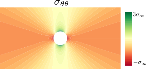
The \(\sigma_{\theta\theta}\) stress is positive for \(\pi/3<\theta<2\pi/3\) and \(-2\pi/3<\theta<-\pi/3\), and negative elsewhere. The stress \(\sigma_{\theta\theta}\) for \(\theta=\pi/2\) is denoted by \(\sigma_y\)
\[\sigma_y = \sigma_\infty\left(1+\dfrac{1}{2}\dfrac{a^2}{x^2}+\dfrac{3}{2}\dfrac{a^4}{x^4}\right)\]The gradient of stress \(\sigma_y\) along the hole axis
\[\dfrac{d\sigma_y}{dx}= -\sigma_\infty a^2\left(\dfrac{1}{x^3}+\dfrac{6a^2}{x^5}\right), \qquad \dfrac{d\sigma_y}{dx}\biggl|_{x=a}= -7\dfrac{\sigma_\infty}{a}\]At the edge of the hole with r = a,
\[\sigma_{rr}=\sigma_\infty(1-2\cos{(2\theta)})\]The maximum stress around the circle is located at \(\theta = \pi/2\) or \(\theta = 3\pi/2\)
The stress concentration factor, \(K_t\), is the ratio of maximum stress at the hole to the remote stress:
\[K_t = \dfrac{\sigma_{max}}{\sigma_\infty}=\dfrac{\sigma_{\theta\theta}(a,\pm \pi/2)}{\sigma_\infty}=3\]Note that for an infinite plate, the stress concentration factor is independent of the hole size.
Finite Width Effects: for finite width plates, we introduce a nominal stress defined by
\[\sigma_{nominal}=\dfrac{W}{W-2a}\sigma\]
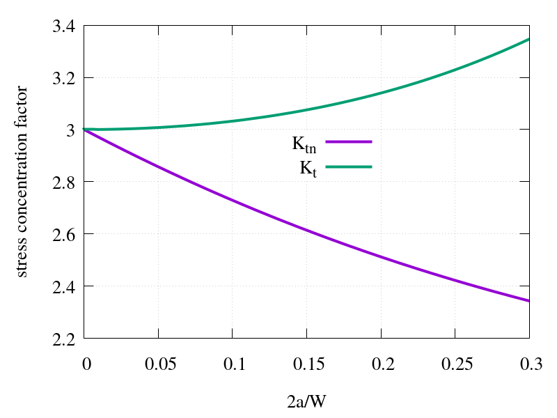
For this case, the stress concentration factor will be defined as \(K_{tn}=\dfrac{\sigma_{max}}{\sigma_{nominal}}\). An empirical formula for \(K_{tn}\) is
\[K_{tn} = 3 - 3.14 \left( {2a \over W} \right) + 3.667 \left( {2a \over W} \right)^2 - 1.527 \left( {2a \over W} \right)^3\]The stress concentration factor \(K_{tn}\) varies between 2 (\({2a\over{W}} \longrightarrow 1\) ) and 3 (\({2a\over W} \longrightarrow 0\)).
Elliptic holes:
The maximum \(\sigma_{\theta\theta}\) stress is given by
\[\sigma_{\theta\theta}^{max}=\sigma_\infty \left(1+2\dfrac{a}{b}\right)\]The stress intensity factor is given by \(K_t=1+2\dfrac{a}{b}\). The gradient of stress along the y-axis
\[\dfrac{d\sigma_y}{dx}\biggl|_{x=a}= -\sigma_\infty \dfrac{a}{b^3}\left(4a+3b\right)\]
Mesh generation#

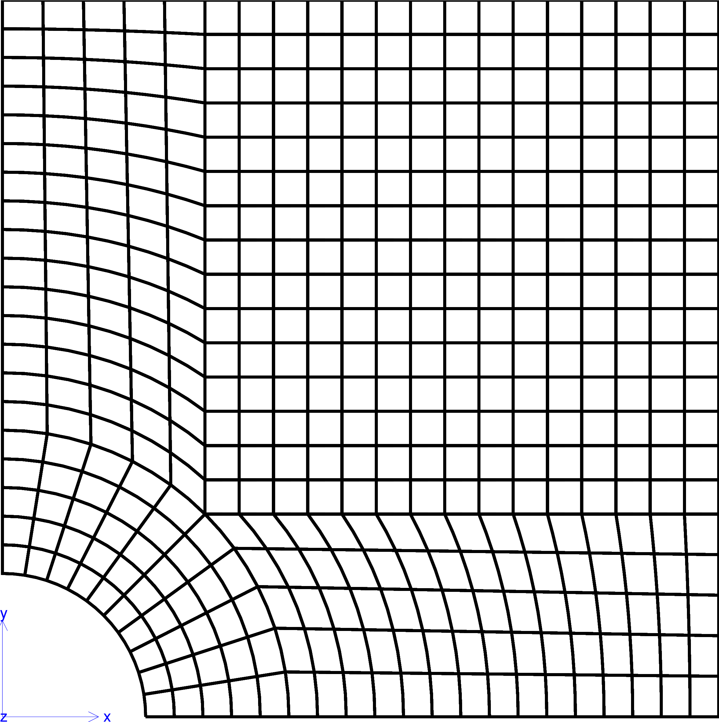
Fig. 47 The geometry of one-quarter of a plate with a hole.#
To create the mesh, two methods are used. The first one uses the Zmaster GUI to create the mesh, while the second one is based on a specific “mesher” developed to generate this kind of meshes. The second way is useful to create the mesh for elliptic hole which is not possible using the Zmaster interface.
Method 1#
To create the mesh of a quarter of a plate with elliptical hole using the Zmaster interface. For a plate having an edge length of 2 mm and circular hole of radius 0.2,
Create points

#Points    X           Y           Z

point0     0.0         0.0         0.0
point1     0.2         0.0         0.0
point2     0.4         0.0         0.0
point3     1.          0.0         0.0
point4     1.          0.282842712 0.0
point5     1.          1.          0.0
point6     0.282842712 1.          0.0
point7     0.0         1.          0.0
point8     0.0         0.4         0.0
point9     0.0         0.2         0.0
point10    0.282842712 0.282842712 0.0
point11    0.141421356 0.141421356 0.0
Create lines
 ,
,#Lines 1st point -- 2nd point line0 point1 -- point2 line1 point2 -- point3 line2 point3 -- point4 line3 point4 -- point5 line4 point5 -- point6 line5 point6 -- point7 line6 point7 -- point8 line7 point8 -- point9 line8 point4 -- point10 line9 point10 -- point6 line10 point11 -- point10
and arcs

#Arcs  1st point  2nd point  center  radius  theta1    theta2

arc0   point1     point11    point0  0.2     0.0       0.785398
arc1   point11    point9     point0  0.2     0.785398  1.570796
arc2   point2     point10    point0  0.4     0.0       0.785398
arc3   point10    point8     point0  0.4     0.785398  1.570796
Create a ruled domain

#domain  element types  boundary
 Ruled0  c2d8r          arc0   line10  arc2    line0
 Ruled1  c2d8r          arc1   line7   arc3    line10
 Ruled2  c2d8r          arc2   line8   line2   line1
 Ruled3  c2d8r          line8  line9   line4   line3
 Ruled4  c2d8r          arc3   line6   line5   line9
Specify the number of nodes at each edge
 (the number of nodes at opposite sides
should be the same)
(the number of nodes at opposite sides
should be the same)Create boundary sets

#Bsets     Boundary

x0         line7 -- line6
x1         line2 -- line3
y0         line0 -- line1
y1         line5 -- line4
hole_egde  arc0  -- arc1
Mesh the domain

Method 2#
Alternatively, the mesh can be created using the **mesh_quarter_plate_hole mesher, which
enables the creation of a mesh based on multiple parameters ( plate edge length, hole radius, …)
as shown below:
% file mesh_plate.inp
****mesher
 ***mesh plate_circular_hole.geof
  **mesh_quarter_plate_hole
   *ncut_radius 20                  % number of elements in radial-direction
   *ncut_theta  30                  % number of elements in theta-direction
   *size_square 1.00                % plate edge length / 2
   *size_hole 0.2                   % radius a
   *nb_reg 3                        % number of mesh layers with the same hole roundness
   *quad                            % quadratic mesh
   *geometrical_progression 1.1     % mesh progression in radial direction,
                                    % finer mesh near the hole
   *hole_anisotropy 1.              % aspect ratio b/a , 1 = hole is circular
   *balance_nodes

  % the following bset are required for calcul and post-processing
  **bset x0 *use_nset x0
  **bset y0 *use_nset y0
  **bset x1 *use_nset x1
  **bset y1 *use_nset y1
  **rename_set *nsets layer_0  hole_edge
  **bset hole_edge *use_nset hole_edge
 **set_reduced                      % reduced integration
****return
To run this mesher, open a terminal and execute
> Zrun -m mesh_plate.inp
This will create plate_circular_hole.geof mesh file, which can be visualized using the command
> Zmaster plate_circular_hole.geof
and then click on  .
.

Finite element analysis#
The input file to perform a finite element computation
Finite element formulation#
****calcul mechanical
  ***mesh plane_stress
   **file plate_circular_hole_4.geof
Global problem resolution#
***resolution
 **sequence
  *time 1.
  *increment 1
Boundary conditions#
The following boundary conditions are applied:
For symmetry, the displacement of
x0along x-direction andy0along y-direction is set to 0.Apply a tensile loading using
**pressureon the bsetx1, with \(P^{\tt x1}(t)=100t\).
***bc
 **impose_nodal_dof
   x0 U1 0.0
   y0 U2 0.0
 **pressure x1 100. time
Material behavior#
The material behavior file and the integration method (required for plastic models) are specified as
***material
  *file elastoplastic.mat                  % or elastic.mat
  *integration theta_method_a 1. 1e-12 100 % this is not required for an elastic model
Elastic material behavior
% elastic.mat file
***behavior gen_evp
 **elasticity isotropic
   young 200000.
   poisson 0.3
***return
Elastoplastic material behavior
 % elastoplastic.mat file
 ***behavior gen_evp
  **elasticity isotropic
    young 200000.
    poisson 0.3
  **potential gen_evp ep
   *flow plasticity
   *criterion mises
   *isotropic constant
    R0 300.
***return
Output results#
The value of stress components \(\sigma_{11}\), \(\sigma_{22}\) and \(\sigma_{12}\) along
the boundary lines x0, y0 and hole_edge can be output in ASCII files (one file for each
liset as):
***output
 **curve stress_x0.test
  *liset_var x0 X Y sig11 sig22 sig12
 **curve stress_y0.test
  *liset_var y0 X Y sig11 sig22 sig12
 **curve stress_edge.test
  *liset_var hole_edge X Y sig11 sig22 sig12
Note that the stress values are extrapolated to line set (liset) nodes.
Post-processing#
The following input file allows to apply a series of post-processing steps:
**process transform_frame: compute stress tensor components in the cylindrical coordinate system. It will create variables namedsig11-rot, …,sig12-rot.**process node_extrapolation: extrapolate the values of stress in cylindrical coordinates to nodes. Here we extrapolate onlysig11-rotandsig22-rot(the output names for the newly created nodal variables are chosen to besig_rr,sig_tt, respectively).**process gradient: compute the gradient of a stress component (e.g. \(\dfrac{\partial \sigma_{\theta\theta}}{\partial Y}\)). The name of this variable isgradYsig_tt.**process node_extrapolation: extrapolate the value of the stress gradient to nodes. The name of the corresponding nodal variable is chosen asNgradYsig_tt.**process format: export the specified variables at specified maps to an output ASCII file.
****post_processing
 ***global_post_processing
% **output_number 1
%-------------------------------------
  **file integ
  **elset ALL_ELEMENT
  **process transform_frame
   *local_frame cylindrical
    (0. 0. 0.) (0. 0. 1.)
   *tensor_variables sig
%-------------------------------------
  **process node_extrapolation
   *list_var    sig11-rot sig22-rot % the name of the field to be extrapolated
   *output_var  sig_rr     sig_tt   % the output name
%-------------------------------------
  **file node
  **nset ALL_NODE
  **process gradient Y *var sig_tt  % this will compute gradYsig_tt = d{sig_tt}/dY
%-------------------------------------
  **file integ
  **elset ALL_ELEMENT
  **process node_extrapolation
   *list_var    gradYsig_tt
   *output_var  NgradYsig_tt
%-------------------------------------
  **file node
  **nset x0           % for example
  **output_number 34  % map number
  **process format
   *file results.dat % output filename
   *list_var sig_rr sig_tt NgradYsig_tt
   *write_nodal_coordinates coord
****return
To run this post-processing, execute
Zrun -pp plate_tension1.inp
The variables computed by these post-processings are stored in the plate_tension1.integp/plate_tension1.nodep files.
Results & discussion#
In this section, finite element solutions will be compared to analytical solution for isotropic elasticity and for elasto-plasticity. The case of uni-axial and bi-axial tensile loading is addressed.
Isotropic elasticity#
Uni-axial tensile loading (circular hole)
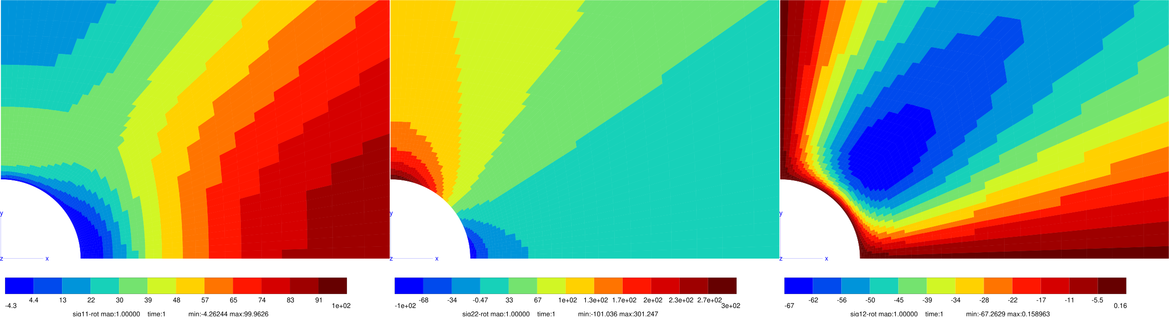
Fig. 48 Finite element solution for \(\sigma_{rr}\) (left), \(\sigma_{\theta\theta}\) (middle), and \(\sigma_{r\theta}\) (right).#
Bi-axial tensile loading (circular hole)
For infinite plate with a circular hole, the solution can be derived by superposing the solutions of uni-axial tensile loading obtained for \(\theta\) and \(\theta+\pi/2\).

We denote by \(\alpha = \dfrac{\sigma_\infty^2}{\sigma_\infty^1}\). The stress concentration factors at points A and B are given by:
\[K_t^A=3\alpha-1, \qquad ~K_t^B=3-\alpha\]When \(\sigma_\infty^1\) and \(\sigma_\infty^2\) have the same magnitude but are of opposite sign (pure shear \(\alpha=-1\)), \(K_t^A=-4, \text{and}~K_t^B=4\).
To apply a bi-axial stress, one can modify the input file as
***bc
 **impose_nodal_dof
   x0 U1 0.0
   y0 U2 0.0
 **pressure x1 100. time
            y1 100. time % for alpha = 1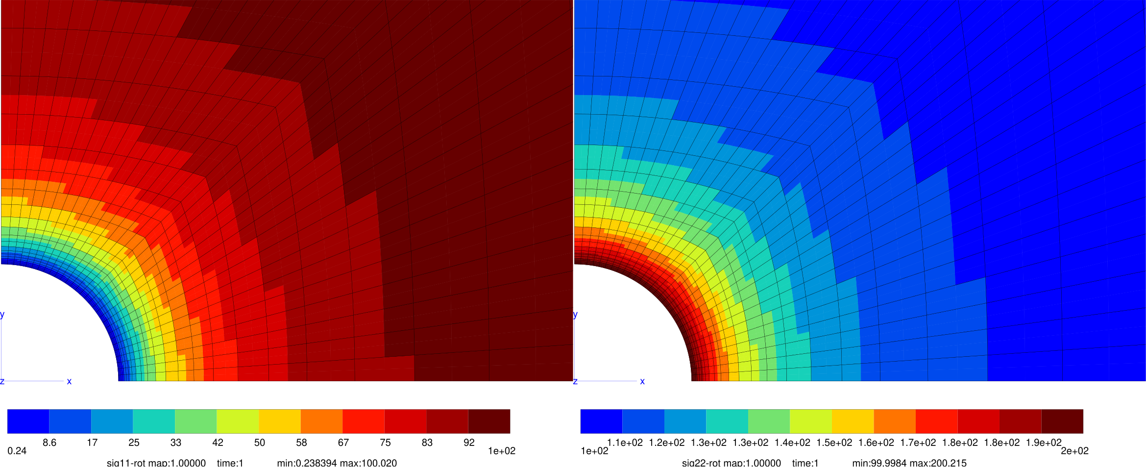
Fig. 49 Finite element solution for \(\alpha=1\): \(\sigma_{rr}\) (left) and \(\sigma_{\theta\theta}\) (right). The stress \(\sigma_{r\theta}\approx 0\).#
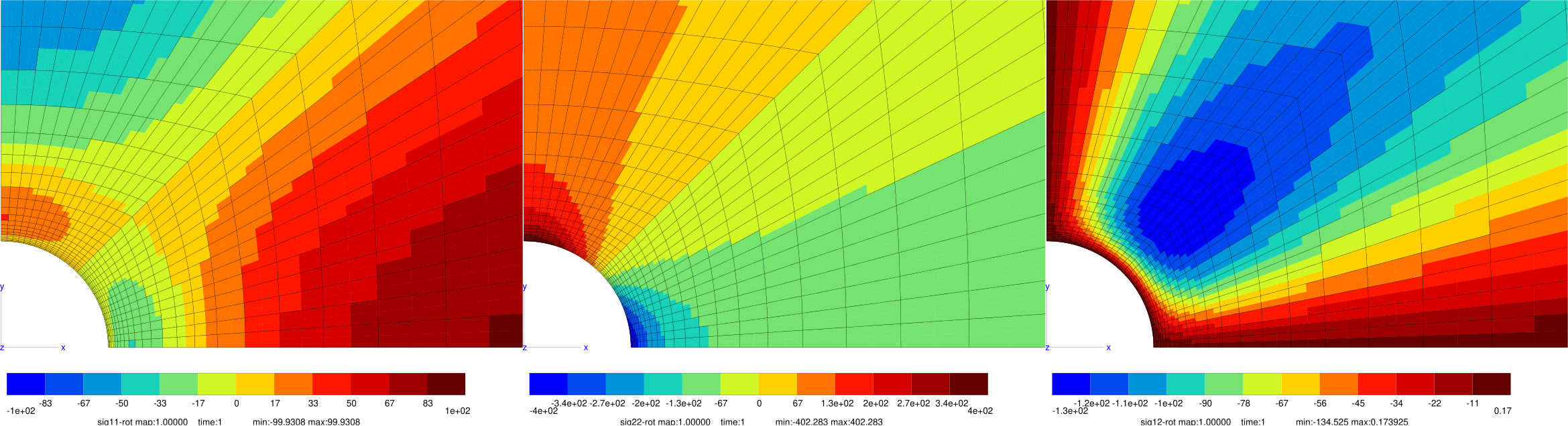
Fig. 50 Finite element solution for \(\alpha=-1\): \(\sigma_{rr}\) (left), \(\sigma_{\theta\theta}\) (middle), and \(\sigma_{r\theta}\) (right).#
The finite element results agree perfectly with the analytical solution.
Elliptical hole
For a infinite plate with an elliptic hole subjected to uni-axial loading, the stress concentration factor is of \(K_t=1+{2a \over b}\). For biaxial loading (\(\alpha=1\)), \(K_t ={2a \over b}\). Finite element results are slightly different because the plate has a finite width.
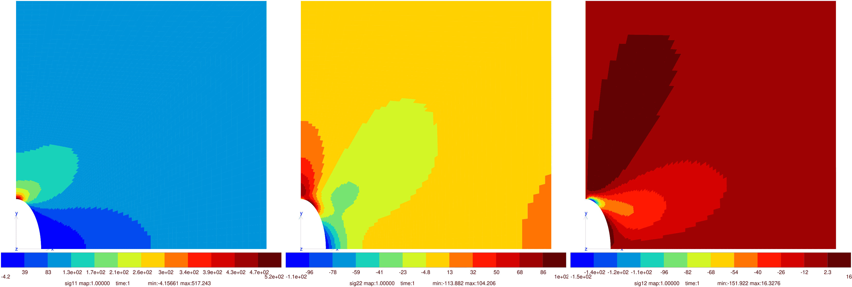
Fig. 51 Finite element solution for a plate with an elliptic hole subjected to uni-axial loading.#
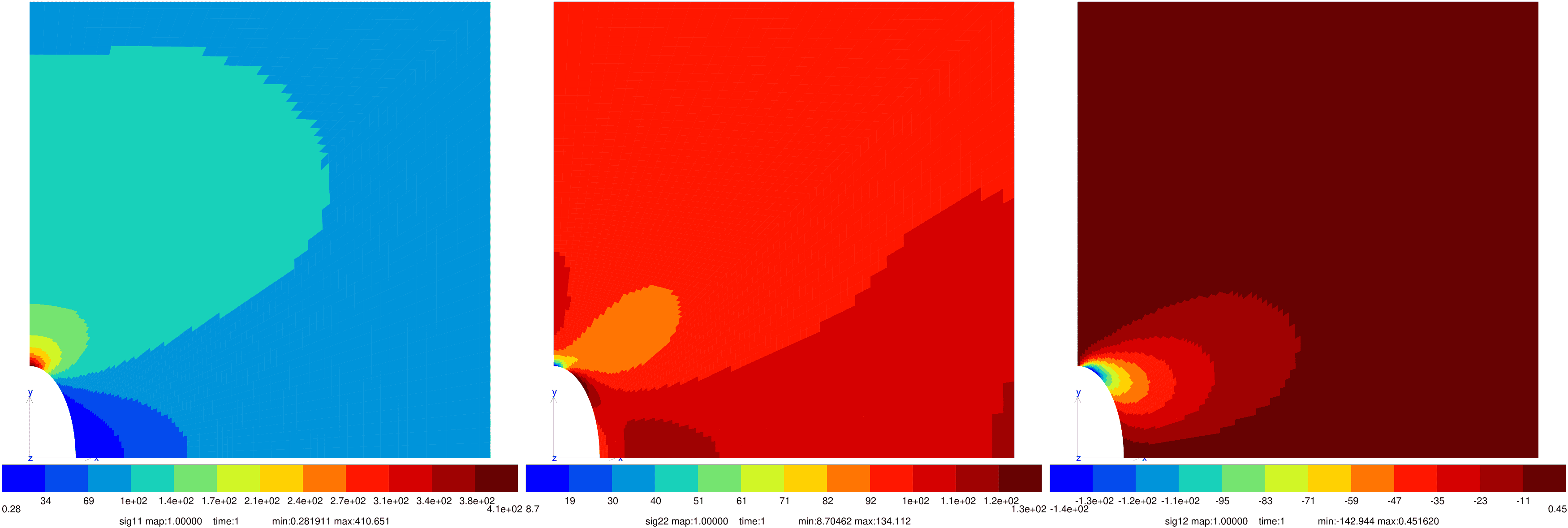
Fig. 52 Finite element solution for a plate with an elliptic hole subjected to bi-axial loading.#
Elasto-plasticity#
Now, we assume that the material is elasto-plastic, and consider a biaxial loading (\(\alpha=1\)) with \(\sigma_\infty = 200 MPa\).
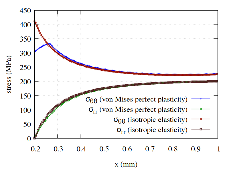
Fig. 53 Comparison of finite element results (\(\sigma_{rr}\) and \(\sigma_{\theta\theta}\)) for an isotropic elastic model and a perfect von Mises plasticity model (\(R_0 = 300\) MPa).#
Downloads
Mesh files
Input files