Elastoplastic analysis of a tube under pressure#

Highlights

Mesh a 2D geometry using Zmaster GUI
Create the material file input using Zair GUI
Create the input file using Zair GUI
Launch and visualize the results of a finite element computation
Compute the strain/stress components at the cylindrical coordinates
Output results in ASCII files

Problem specification#

The study proposed in this tutorial focuses on the analysis of an infinite tube under internal pressure. This tube is subjected to a uniform internal pressure of \(P = 60 MPa\). Since it is an infinite tube, a two-dimensional model will be considered which consist of a cross-sectional slice.

The Finite Element modeling will be performed using plane strain conditions. Due to the geometric and loading symmetries of the structure, only a quarter of the thick tube’s cross-section will be modeled.

../../_images/model.svg — Fig. 41 The quarter of the thick tube’s cross-section#

Table 2 Loading, geometry and material parameters#
Parameters	Numerical value
internal pressure	60 MPa
yield stress \(\sigma_0\)	100 MPa
inner radius \(R_i\)	100 mm
outer radius \(R_e\)	200 mm
Young’s modulus	205000 MPa
Poisson’s coefficient	0.3
density	8.08e-9 kg/mm\(\,\!^3\)

Analytical solutions#

The analytical solution of this problem is given in [T1].

In the plastic region (\(R_i \leq r \leq c\)):

\[\begin{split}\begin{aligned} \sigma_{rr} &= - \dfrac{\sigma_0}{\sqrt{3}} \left( 1 - \dfrac{c^2}{R_e^2} + 2 \ln \left( \dfrac{c}{r} \right) \right) \\ \sigma_{\theta\theta} &= \dfrac{\sigma_0}{\sqrt{3}} \left( 1 + \dfrac{c^2}{R_e^2} - 2 \ln \left( \dfrac{c}{r} \right) \right) \\ \sigma_{zz} &= \nu \left( \sigma_{rr} + \sigma_{\theta\theta} \right)\qquad (\text{plane strain}) \end{aligned}\end{split}\]

In the elastic region (\(c \leq r \leq R_e\)):

\[\begin{split}\begin{aligned} \sigma_{rr} &= - \dfrac{\sigma_0}{\sqrt{3}} \dfrac{c^2}{R_e^2} \left( \dfrac{R_e^2}{r^2} - 1 \right)\\ \sigma_{\theta\theta} &= \dfrac{\sigma_0}{\sqrt{3}} \dfrac{c^2}{R_e^2} \left( \dfrac{R_e^2}{r^2} + 1 \right)\\ \sigma_{zz} &= \nu \left( \sigma_{rr} + \sigma_{\theta\theta} \right) \qquad (\text{plane strain}) \end{aligned}\end{split}\]

Mesh generation#

To create the tube geometry with Zmaster:

Run the command Zmaster tube.mast in a terminal to open the Zmaster interface. This command will create a file tube.mast in which the geometry will be stored in text form.
Click on \(\longrightarrow\) to create the points that define the geometry, which in this case is a quarter of a disk.

Enter the coordinates of a point (X, Y, Z), then click GO to create the point. Repeat the process for all points.

#Points      X         Y         Z
      100.       0.        0.
      200.       0.        0.
       0.       200.       0.
       0.       100.       0.
       0.        0.        0.

Click on View, Auto-center to view all points.
Click on \(\longrightarrow\) to create lines

Choose 2 points, then click Go.

Click on points 1 and 2 to define line 1, which will be created.

Next, click on points 3 and 4 to define line 2 and create it.
To create the inner and outer circular arcs, click on \(\longrightarrow\) . In the Create Arc window, select Arc: center, pt1, pt2 to create the arcs using the center and two points, then confirm with OK.

Click on the center point no. 5 (0,0,0) then point no. 1 and point no. 4 to create the inner arc.

Click on the center point no. 5 (0,0,0) then point no. 2 and point no. 3 to create the outer arc.
Save the progress by clicking on File, Save.

Note

All these steps help to populate the tube.mast file. If you open it with a text editor, you will notice that there is a section for each created entity (points, lines, arcs).
You can achieve the same result by writing the keywords for each entity and opening it with the command Zmaster tube.mast to visualise the result.
You can modify the properties of the created entities directly in the tube.mast file, for example, it is possible to change the coordinates of the points, the radii of the arcs, etc.

The content of the tube.mast file:

****master
 ***geometry
  **point point0
   *position 1.000000000000000e+02 0.000000000000000e+00 0.000000000000000e+00
  **point point1
   *position 2.000000000000000e+02 0.000000000000000e+00 0.000000000000000e+00
  **point point2
   *position 0.000000000000000e+00 2.000000000000000e+02 0.000000000000000e+00
  **point point3
   *position 0.000000000000000e+00 1.000000000000000e+02 0.000000000000000e+00
  **point point4
   *position 0.000000000000000e+00 0.000000000000000e+00 0.000000000000000e+00
  **line line0
   *p1 point0
   *p2 point1
  **line line1
   *p1 point2
   *p2 point3
  **arc arc0
   *p1 point0
   *p2 point3
   *center point4
   *data   1.000000000000000e+02 0.000000000000000e+00 1.570796326794897e+00
  **arc arc1
   *p1 point1
   *p2 point2
   *center point4
   *data   2.000000000000000e+02 0.000000000000000e+00 1.570796326794897e+00
 ***plotting
  **default_options 1 0 1
****return

Structure meshing#

To mesh the previously created geometry, follow these steps:

If the Zmaster interface is closed, open the geometry file using the command Zmaster tube.mast.
Start by specifying the desired number of nodes on the geometry boundaries (inner and outer) by clicking on \(\longrightarrow\) , and entering the desired number of nodes for each boundary. Each pair of opposite sides must have the same number of nodes (for example, 20 for both opposite lines and 40 for both opposite arcs).
Before meshing the quarter of the disk, you must choose the desired mesh type: structured or free.
1. In the case of a structured mesh:
  - Click on \(\longrightarrow\) .
  - Choose the element group name Elset, element type (c2d), linear or quadratic elements Quadratic, normal or reduced integration Normal and, since the mesh contains two linear sides, Sides 2 4 linear.
  - Click Start, then select the boundaries in an order such that the lines are numbered 2 and 4 (for example, in this order: 1-inner arc, 2-line #1, 3-outer arc, and 4-line #2).
  - Click on \(\longrightarrow\) to mesh the geometry.
  - Click on to show the mesh.
2. In the case of a free mesh:
  - Click on \(\longrightarrow\) .
  - Choose the Elset name, element type (c2d), linear or quadratic elements, normal or reduced integration, and Delaunay Triangles.
  - Click Start, then select the boundaries (no specific order required for the lines).
  - Click on \(\longrightarrow\) to mesh the geometry.
  - Click on to show the mesh.

Note

All these steps populate the tube.mast file and create a tube.geof file, which contains all the nodes and elements of the created mesh.
If you open the tube.mast file with a text editor, you will notice that additional sections have been added, defining the meshing domain and the type of mesh (structured or free) and the number of nodes in each entity: lines (*cuts 20) and arcs (*cuts 40).
You can obtain the mesh file tube.geof by adding the previous sections and running the command Zrun -B tube.mast in a terminal.
You can modify the mesh characteristics in tube.geof directly from the tube.mast file; for example, it is possible to change the number of nodes for each entity with (*cuts 20), the type of elements, etc. Then, run the command Zrun -B tube.mast to create the mesh in the tube.geof file.

Additional sections in the tube.mast file :

**domain domain1 Ruled0
 *name R
 *element c2d8
 *method 1
 *b1 arc0
 *b2 line0
 *b3 arc1
 *b4 line1

Modified sections :

**line line0
 *p1 point0
 *p2 point1
 *cuts 20     % added line

**arc arc0
 *p1 point0
 *p2 point3
 *cuts 40     % added line
 *center point4
 *data   1.000000000000000e+02 0.000000000000000e+00 1.570796326794897e+00

The content of the tube.geof file:

***geometry
 **node
  2521 2
  1 -3.828568698926949e-14 1.000000000000000e+02
  2 3.925981575906801e+00 9.992290362407230e+01
  …
 **element
  800
  1 c2d8 1 44 2 48 43 166 42 45
  2 c2d8 2 47 3 51 46 169 43 48
  …
***group
 **elset R
  1 2 3 4 5 6 7 8 9 10 11 12 13 14 15 16 17 18 19 20 21
  …
***return

Creation of nsets, bsets, or elsets

It will be useful to create groups of nodes (nsets), boundary groups (bsets), or element groups (elsets) to apply boundary conditions or to plot stress along a line, for example, to easily apply boundary conditions, groups of nodes will be created.

==========  =======================
Nsets       Definition
==========  =======================
left        x<0.001
bottom      y<0.001
inner_wall  x*x+y*y<100.*100.+0.001
outer_wall  x*x+y*y>200.*200.-0.001
==========  =======================

The steps to define nsets and bsets from nsets :

Click on \(\longrightarrow\) , then on nset. Enter the name of the nset, the function defining the nset, and then confirm with OK. Repeat this operation for as many nsets as needed.
Click on \(\longrightarrow\) , then on bset_from_nset. Enter the name of the nset, and then confirm with OK. Repeat this operation for as many bsets created from the nsets.

Click on \(\longrightarrow\) , then save the mesh using File \(\longrightarrow\) Save.

Note

If you open the file ‘tube.mast’ with a text editor, you will notice that there are additional sections that have been added, defining the nsets, bsets, or elsets.
If you want to modify this part, for example, the function for an nset, simply use the command ‘Zrun -B tube.mast’ to create the nsets and bsets or elsets.

The additional sections in the tube.mast file:

***mesher
 **nset
  *type cartesian
  *name left
  *axes 0 1 2
  *limit 0.00100000
  *func x<0.001 ;
 **nset
  *type cartesian
  *name bottom
  *axes 0 1 2
  *limit 0.00100000
  *func y<0.001 ;
 **nset
  *type cartesian
  *name inner_wall
  *axes 0 1 2
  *limit 0.00100000
  *func x*x+y*y<100.*100.+0.001;
 **nset
  *type cartesian
  *name outer_wall
  *axes 0 1 2
  *limit 0.00100000
  *func x*x+y*y>200.*200.-0.001;
 **bset_from_nset
  *nset_name left
 **bset_from_nset
  *nset_name bottom
 **bset_from_nset
  *nset_name inner_wall
 **bset_from_nset
  *nset_name outer_wall

In order to view the nsets, bset and the elsets, click on , a window will open that contain three list :
- the first is for the nsets,
- the second is for the bsets,
- the third is for the elsets.
Select the entity to view and then click on Draw.

Finite element analysis#

Problem definition#

The problem definition, solution method, boundary conditions, and loads are defined in the tube.inp file using an Auto_reader interface.

Type the command Zmaster tube.inp in a terminal to create the file where the problem data will be stored.
Click on Options, then Auto reader. A window containing the interface will open.
Click on problem, use Filter selection to search for calcul_mechanical, then select this option and confirm with Set. A tree structure will open below problem, containing all the parameters for defining a mechanical calculation.
Start by defining the mesh that will be used by clicking on mesh_def [...] under mesh, select file, and confirm with Set. Click on file that will appear under mesh_def [...] and enter the name of the mesh file, then validate with Open. Click on default_type and choose plane_strain.
Click on resolution to define the parameters of the solution algorithm. Select void and confirm with Set. A tree structure will appear under void and resolution. Click on sequences [+-], choose sequence, then click on Add and enter the following values for the different parameters under sequence:
- nb sequences => 1
- time => 1.0
- increment => 10
- iteration => 5
- algorithm => p1p2p3 (update tangent stiffness at each iteration)
- ratio:
- type => relative (default): residual divided by the norm of external reaction
- value => 1.e-06
- symmetrize => True
To define the boundary conditions and loads applied to the structure, click on bcs [+-], choose impose_nodal_dof using Filter selection, and confirm with Add.

Select the options below to constrain the displacement on the bottom nset in the vertical direction:
- group (*) => bottom
- dof (*) => U2
- handler => void => coefficients => 0.0
Select the options below to constrain the displacement on the left nset in the horizontal direction:
- group (*) => left
- dof (*) => U1
- handler => void => coefficients => 0.0
To define the loads applied to the structure, click on bcs [+-], and choose pressure.

Select the options below to apply the load on the inner wall nset in the vertical direction:
- group (*) => outer wall
- handler => void:
- coefficients => -60.0
- tables => tab
Click on table [+-], choose name, and confirm with Add. A tree structure will appear under tables, allowing you to define the evolution of the load over time in the tab table. Select the options below:
- name => tab
- time => 0.0 1.0
- value => 0.0 1.0
Add the previously created material file perfectly_plastic.mat by clicking on file_name (*) under file and material. Click on ... and select the perfectly_plastic.mat file, then confirm with Open twice.
Save the problem definition by specifying the file name tube.inp and clicking the Write button. A tube.inp file will be created containing the problem data.

The content of the tube.inp file:

****calcul
 ***table
   **name tab
     *time 0.00000 1.00000
     *value 0.00000 1.00000
 ***mesh plane_strain
   **file tube.geof
 ***resolution
   **sequence 1
     *time 1.00000
     *increment 5
     *iteration 10
     *algorithm p1p2p3
     *ratio 1.00000e-06
   **symmetrize
 ***bc
   **pressure
     inner_wall  -60.0000 tab
   **impose_nodal_dof
     bottom U2  0.00000
     left U1  0.00000
 ***material
     *file perfectly_plastic.mat
****return

Material behavior#

To assign a material to the created mesh, follow these steps:

Click on Options, then Behavior reader. A window opens allowing you to define the material.
Modify the name of the output file by entering something like perfectly_plastic.mat. Choose gen_evp and click on Set. A tree structure will appear on the left side containing the various parameters to define.
Select elasticity from the tree structure, then choose the type of elasticity, for example, isotropic. Then, click on Set. The Young’s modulus and the Poisson’s ratio will be added to the tree structure under isotropic and elasticity.
Click on young(*) to define the Young’s modulus, then choose the application method for the modulus, such as constant, and confirm with Set. Constant will be added below Young. By clicking on constant, the value can be defined.
The Poisson’s ratio is defined in the same way, with a value of 0.3.
To define the material’s density, simply click on the parameter masvol below coefficient, then choose constant, confirm with Set, and finally enter the coefficient value as 8.08000e-09.
To achieve perfectly plastic behavior, start by defining the potential by clicking on it, choose gen_evp from the list, and then click on Add. The potential gen_evp will be added to the tree structure.
You need to define the new parameters under gen_evp:
- name => ‘ep’,
- criterion (*) => ‘mises’ and confirm with Set,
- flow (*) => ‘plasticity’ and confirm with Set,
- isotropic => ‘constant’,
- R0 => ‘constant’,
- constant => ‘100.0’
Specify the name of the file to something more descriptive, like perfectly_plastic.mat. in the Output file section, then save the material behavior by clicking the Write button. A file named perfectly_plastic.mat will be created in the same folder.

Note

All the parameters that have been defined are saved in the file perfectly_plastic.mat.
It is possible to define the material behavior directly without using the interface by entering the keywords and parameter values in this file with a text editor.
You can load a material file in the Behavior_reader interface by clicking on ... to select the file to load, then confirm with Open, and finally click on Load.

The content of the perfectly_plastic.mat file:

***behavior gen_evp
 **potential gen_evp ep
  *criterion mises
  *flow plasticity
  *isotropic constant
   R0  100.00
 **elasticity isotropic
   young  205000.
   poisson  0.300000
 **coefficient
   masvol  8.08000e-09
***return

Note

You can plot the stress-strain curve by using the command Zsim perfectly_plastic.mat in a terminal in the same location as the perfectly_plastic.mat file.

Resolution#

Click on , a window will open containing the command Zrun tube and select Finite element, then click on Go to start the calculation.
It is also possible to start the calculation using a terminal by entering the following command: Zrun tube.inp.

Post-processing#

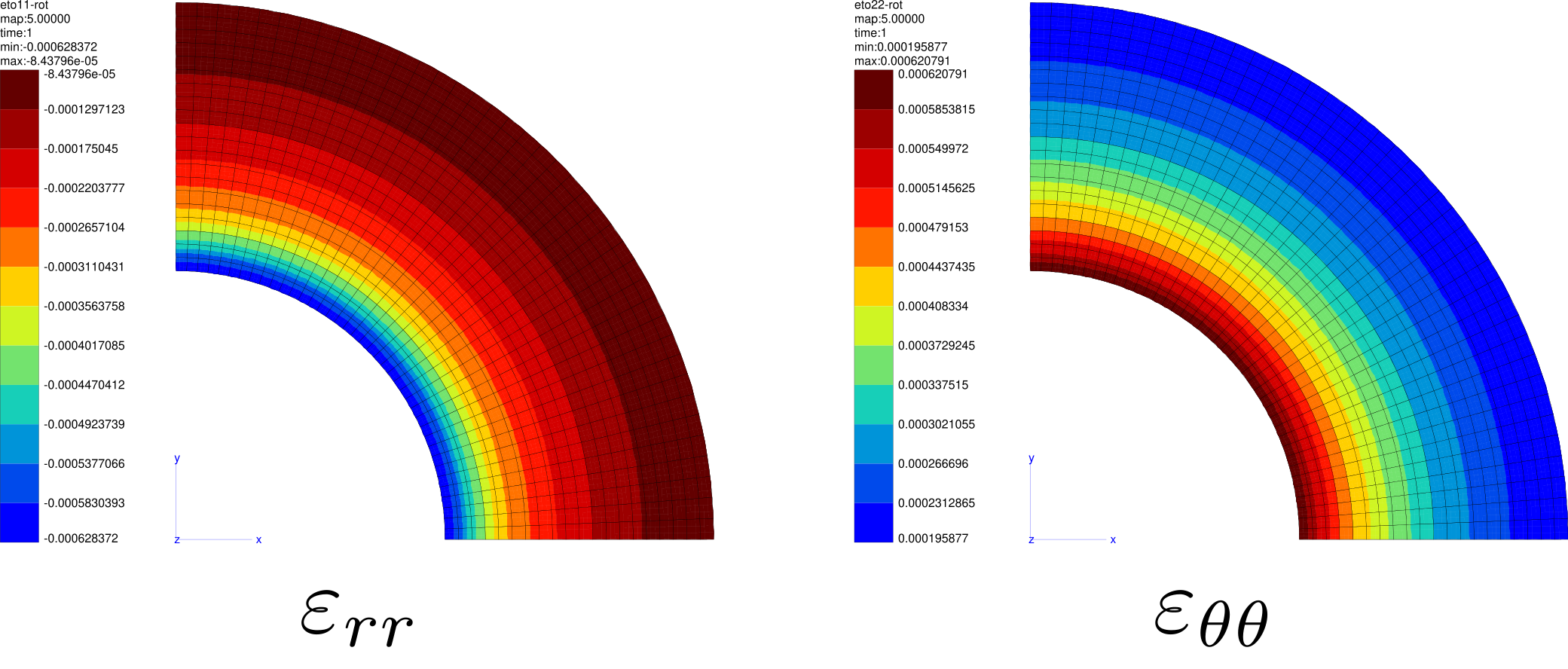
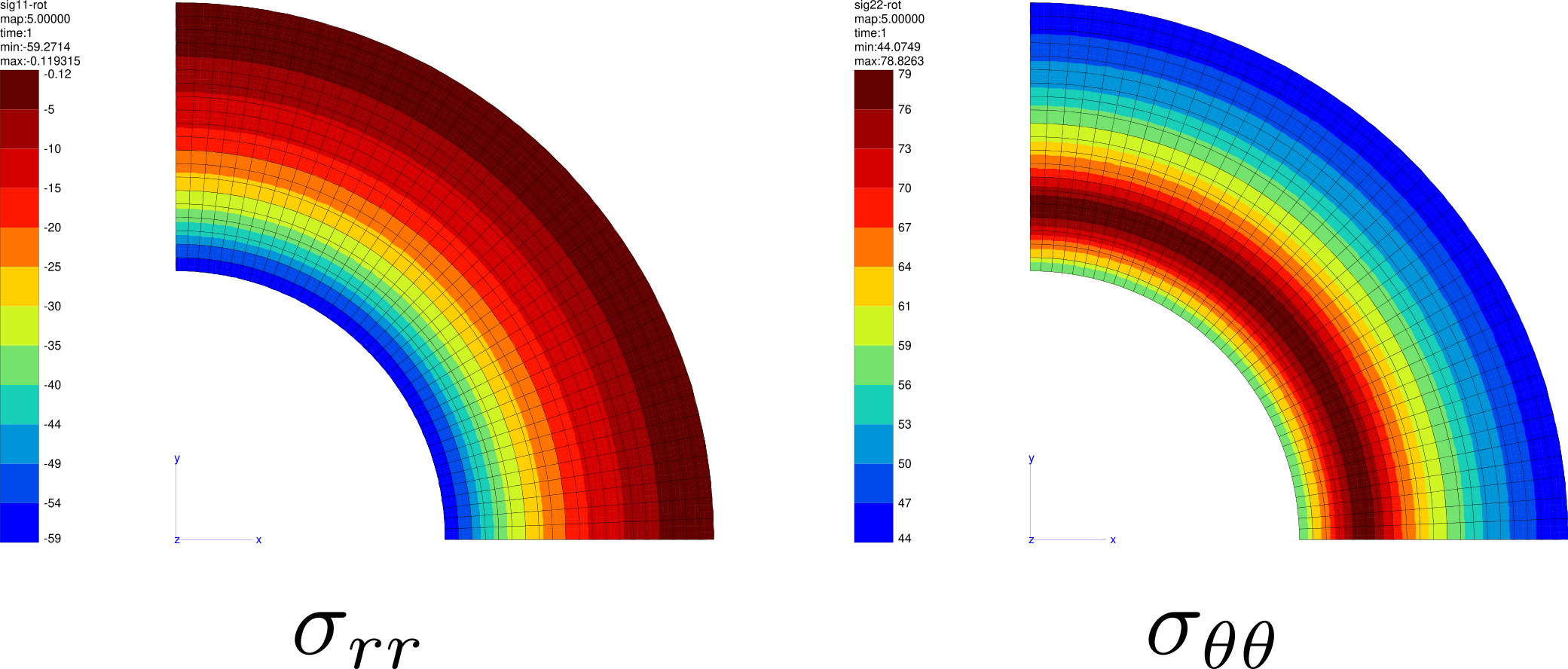
Post-processing of results in a cylindrical local coordinate system

In order to get stress values in the cylindrical coordinates, one can use the following post-processing by adding it at the end of the tube.inp and use the terminal command Zrun -pp tube.inp to run it:

****post_processing
 ***global_post_processing
  **file integ
  **output_number 1-5
  **process transform_frame
   *local_frame cylindrical
    (0. 0. 0.) (0. 0. 1.)
   *tensor_variables sig
   *tensor_variables eto
****return

Results & discussions#

To display the results:

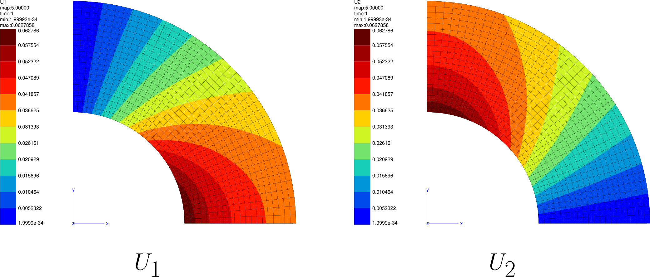
Click on , a Results window will appear containing displacements (U1, U2), reaction forces (RU1, RU2), which are node results. It also includes stresses (sigmises, sig11, sig22, etc.) and strains (epcum, eto11, eto22, etc.) which are results calculated at Gauss points.
Select the result you wish to display, then click Draw or double-click to display the desired result on the mesh.

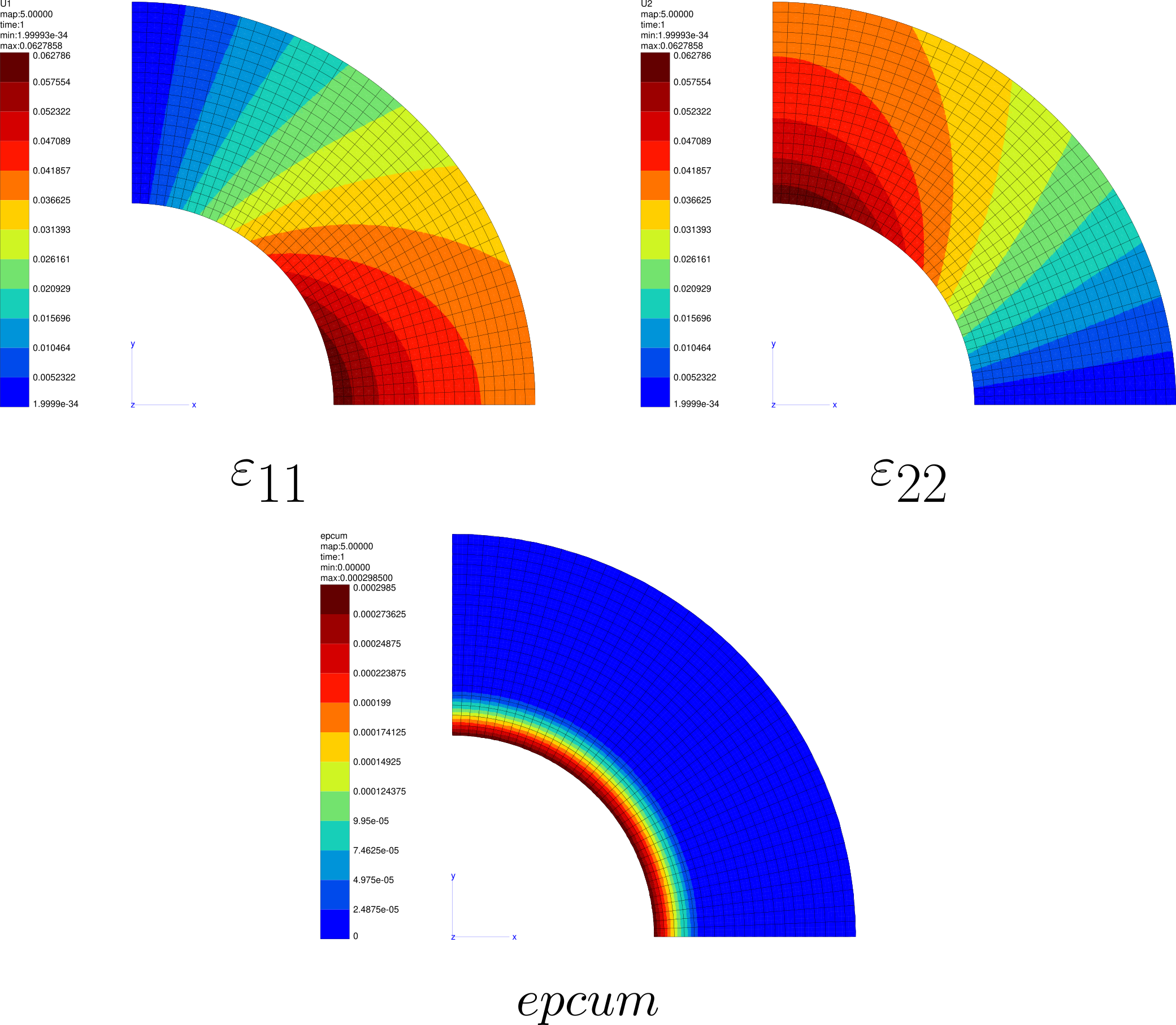
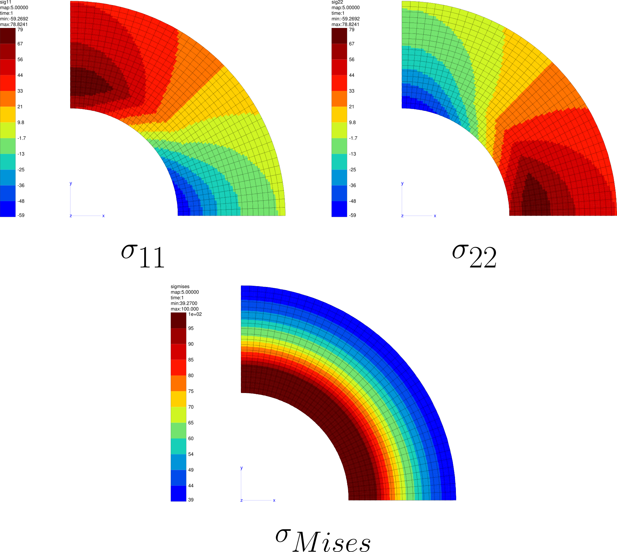
Some examples of calculation results

Displacement Results:

Strain Results:

Stress Results:

Strain Results:

Stress Results:

Comparison with analytical results

When tube having a well-defined yield point is strained by a radial pressure, the strains in the external portion of the tube will be elastic while in the yielded portion next to the internal portion of the tube they will be the sum of an elastic and plastic strain.

Let’s consider \(r=c\) refers to the interface between the plastic region and the elastic region. The position of the interface between plastic and elastic regions : \(c = 125 mm\).

The Finite element stresses function of the radius \(r\) can be extracted from the results along the bottom liset and saved in a text file called sig-rot_bottom.txt using the following post-processing.

The post-processing can be saved in a different file than tube.inp, for example in a file called post.inp.

It will be launched using the terminal command Zrun -pp post.inp:

****post_processing
 ***suppress_p_on_post_files
 ***data_source Z7
  **open tube.ut
 ***precision 3

 ***global_post_processing
 **output_number 5
 **file node
 **nset bottom
 **process curve sig-rot_bottom.txt
  *liset bottom X sig11-rot sig22-rot sig33-rot
****return

First yielding in a tube with an ideally plastic behavior under an internal pressure \(p = 60 MPa\) during the loading phase at the pressure \({p_{first-yield}}_{analytical}\):

\[{p_{first-yield}}_{analytical} = \dfrac{\left( 1 - \dfrac{R_i}{R_e}^2 \right) \sigma_0}{\sqrt{3+(1-2\nu)^2\dfrac{R_i}{R_e}^4}} = 43.22 MPa\]

The curves of cumulated plasticity \(epcum\) and radial stress \(\sigma_{rr}\) for each increment can be extracted from the results along the bottom liset and saved in different text files for each increment called sig-rot_bottom_first-yield_1.txt … sig-rot_bottom_first-yield_5.txt using the following post-processing.

The post-processing can be saved in a different file than tube.inp, for example in a file called post_first-yield.inp.

It will be launched using the terminal command Zrun -pp post_first-yield.inp:

****post_processing
 ***suppress_p_on_post_files
 ***data_source Z7
  **open tube.utp
 ***precision 3

 ***global_post_processing
 **output_number 1
 **file node
 **nset bottom
 **process curve sig-rot_bottom_first-yield_1.txt
  *liset bottom X epcum sig11-rot

 ***global_post_processing
 **output_number 2
 **file node
 **nset bottom
 **process curve sig-rot_bottom_first-yield_2.txt
  *liset bottom X epcum sig11-rot

 ***global_post_processing
 **output_number 3
 **file node
 **nset bottom
 **process curve sig-rot_bottom_first-yield_3.txt
  *liset bottom X epcum sig11-rot

 ***global_post_processing
 **output_number 4
 **file node
 **nset bottom
 **process curve sig-rot_bottom_first-yield_4.txt
  *liset bottom X epcum sig11-rot

 ***global_post_processing
 **output_number 5
 **file node
 **nset bottom
 **process curve sig-rot_bottom_first-yield_5.txt
  *liset bottom X epcum sig11-rot

****return

\[ \begin{align}\begin{aligned}{p_{first-yield}}_{FE} = 47.28 MPa\\{p_{first-yield}}_{analytical} = 43.22 MPa\end{aligned}\end{align} \]

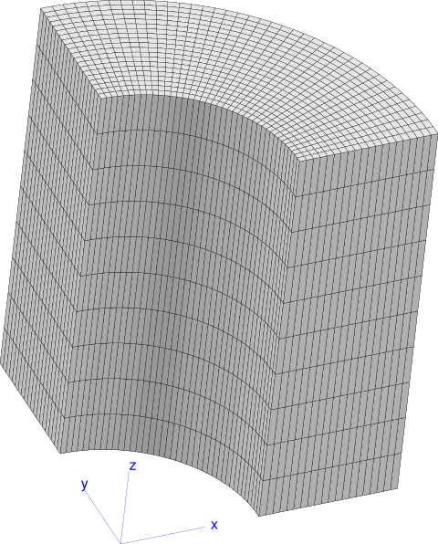
Extension of problem to the 3D case#

Click on \(\longrightarrow\) , then on extension. Enter the name of the elset R, the distance 300.0, the number of elements 10 and then confirm with OK. After that, click on to generate the 3D mesh.

Alternatively, type the following key-words in a file called mesher.inp in order to extrude the 2D geometry along the z axis for a distance of h = 300 mm divided into 10 elements.
```
****mesher
 ***mesh tube_3D.geof
  **open tube.geof
  **extension
   *elset R
   *distance 300.
   *num 10
****return
```
Type in a terminal in the location where you have the files of the problem (.inp, .mat, etc) the command Zrun -m mesher.inp.

A new 3D mesh is created called tube_3D.geof, extra nsets of the existing ones will be created that has the same names with adding the suffix _ext.

These extra nsets are the extrude of the 2D nsets along the z axis.
Add these new bsets from the created new nsets (see Geometry creation) : inner_wall-ext, outer_wall-ext, bottom-ext, left-ext. To do this add the following lines after *num 10 in mesher.inp file :
```
**bset_from_nset
 *nset inner_wall-ext
**bset_from_nset
 *nset outer_wall-ext
**bset_from_nset
 *nset bottom-ext
**bset_from_nset
 *nset left-ext
```

Relaunch the final mesher.inp file in order to create the 3D mesh with the nsets and bsets using the command Zrun -m mesher.inp:

****mesher
 ***mesh tube_3D.geof
  **open tube.geof
  **extension
   *elset R
   *distance 300.
   *num 10
  **bset_from_nset
   *nset inner_wall-ext
  **bset_from_nset
   *nset outer_wall-ext
  **bset_from_nset
   *nset bottom-ext
  **bset_from_nset
   *nset left-ext
  **bset z300
   *func z>299.999;
  **bset z0
   *func z<0.001;
****return

Copy the file tube.inp to create a new file tube_3D.inp, modify these lines :

***mesh plane_strain           =>  ***mesh
 **file tube.geof              =>   **file tube_3D.geof

   inner_wall  -60.0000 tab    =>     inner_wall-ext  -60.0000 tab
   bottom U2  0.00000          =>     bottom-ext U2  0.00000
   left   U1  0.00000          =>     left-ext   U1  0.00000

Add the following lines in the ***bc **impose_nodal_dof section:

z0   U3  0.00000
z300 U3  0.00000

Run the simulation using the command Zrun tube_3D.inp, and visualise the results using the command Zmaster tube_3D.inp.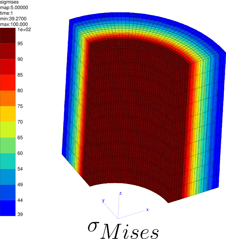

Downloads

Mesh files

tube.mast

mesher.inp
Input files

tube.inp

Elastoplastic analysis of a tube under pressure

On this page

Elastoplastic analysis of a tube under pressure#

Problem specification#

Analytical solutions#

Mesh generation#

Structure meshing#

Finite element analysis#

Problem definition#

Material behavior#

Resolution#

Post-processing#

Results & discussions#

Extension of problem to the 3D case#