Contact between two curved beams#

Highlights

The main objectives of this tutorial are:

To demonstrate how to create a mesh using Zmaster (definition of points, lines, and curves, creation of domains, and the definition of several boundary sets useful for applying boundary conditions).
To create an input file to carry out a large deformations elasto-plastic computation in plane strain conditions. The definition of contact between the two beams is handled for cases with and without friction.
To illustrate how to obtain reaction force values on a set of nodes.

Problem specification#

We consider two contacting curved beams. This problem was introduced by [T5] using a mortar method, and re-addressed by [T6]. One beam is fixed and another is given a horizontal displacement \(d = 32 mm\). Both beams are modelled using a large deformation isotropic hardening elasto-plastic material. The isotropic elasticity properties are given by \(E=689.56\) MPa, and \(\nu=0.32\). The yield stress is \(\sigma_y=31\) MPa, and the plastic modulus is \(H = 261.2\) MPa.

../../_images/geometry2.svg — Fig. 68 The geometry of two curved beams. A displacement \(u_x\) is applied on the top of the upper beam. The lower beam is fixed at the bottom.#

Mesh generation#

To create the mesh using the Zmaster GUI:

Open Zmaster Interface

Create points \(\longrightarrow\)

#Points   x      y     z

point0    0.0    0.0   0.0
point1    10.0   0.0   0.0
point2    12.0   0.0   0.0
point3    -12.0  0.0   0.0
point4    -10.0  0.0   0.0
point5    -15.0  17.0  0.0
point6    -25.0  17.0  0.0
point7    -23.0  17.0  0.0
point8    -5.0   17.0  0.0
point9    -7.0   17.0  0.0

Create arcs
- Select Arc: center, pt1, pt2 \(\longrightarrow\) Go
- Create arcs (in any order). Ensure that the points are selected in an anticlockwise order.
```
#Arcs  center   pt1      pt2

arc0   Point0   point2   point3
arc1   Point0   point1   point4
arc2   Point5   point6   point8
arc3   Point5   point7   point9
```
- Click on Close.

Create lines

Select 2 Points \(\longrightarrow\) Go

Create the following lines (in any order):

#Lines  pt1     pt2

line0   point7  point6
line1   point8  point9
line2   point3  point4
line3   point1  point2

Define the number of nodes at each edge
- Specify the number of nodes on lines in Num field, e.g. 2 (let Progression=1) \(\longrightarrow\) Go.
- Click on the four lines lines.
- Specify the number of nodes on arcs, e.g. Num = 20 \(\longrightarrow\) Go.
- Click on the four arcs.
- Click on Close
Create ruled domains
- Specify the Elset name.
- Select c2d element type, quadratic, Reduced, and Sides 2 4 linear \(\longrightarrow\) Start.
- After selecting the bounding edges of each domain, click on Finish.
```
#Domains     b1   b2    b3    b4

lower_beam   arc1 line2 arc0  line3
upper_beam   arc3 line1 arc2  line0
```
  Ensure that the 2nd and 4th selected edges are lines.
- Click on Close.
Define boundary sets
- Specify Name, select Quadratic, and click on Start.
- Select a boundary set, and click on Finish (after each boundary set)
```
#Bsets      boundaries

lower_bot   line2 line3
upper_top   line1 line0
lower_ext   arc0
upper_ext   arc2
```
- Click on Close.
Mesh the domain
Save the project .mast and the .geof file. (File \(\longrightarrow\) Save)

Finite element analysis#

Finite element formulation#

An updated Lagrangian formulation is used, with plane strain conditions

***mesh updated_lagrangian_plane_strain
 **file curved_beams.geof

Global problem resolution#

One loading sequence (time = 0 to 1) is applied.
A Newton-Raphson algorithm is used, where the tangent matrix is always updated during iterations (p1p2p3).
The number of increments is set to 100, with maximum iterations per increment of 20.
Set automatic time-stepping **automatic_time:
- *divergence 3. 10: to divide time increment by 2 (10 subsequent divergences are allowed).
- *security 1.2: when convergence is retrieved, multiply time increment by 1.2.
- *first_dtime 1e-3: apply a first time increment of 1e-3 for the sequence.

***resolution
 **sequence 1
  *time  1.
  *increment 100
  *iteration 20
  *ratio automatic 0.1
  *algorithm p1p2p3
 **automatic_time epcum 0.1
  *security 1.2
  *divergence 3. 10
  *first_dtime 1e-3

Boundary conditions#

Fix lower_bot node set: the displacement U1 and U2 is set to 0.
Set vertical displacement U2 of upper_top node set to 0.
Apply a horizontal displacement on upper_top as a function of time: \(U_1^{\tt upper\_top}(t)=32t\).

***bc
   **impose_nodal_dof
     lower_bot U1 0.
     lower_bot U2 0.
     upper_top U2 0.
     upper_top U1 32. time

Contact definition#

A mortar contact will be used in this case based on an Augmented Lagrangian method.

Frictionless case:

***mortar_contact
 **interface alm_contact
  *nmortar_side lower_ext
  *mortar_side upper_ext
  *warning_dist 2.

Frictional case:

***mortar_contact
 **interface alm_fric_contact
   *nmortar_side lower_ext
   *mortar_side upper_ext
   *warning_dist 2.
   *fric_coeff 0.3

Material behavior#

Consider an elastoplastic gen_evp model with:

isotropic elasticity,
von Mises plasticity with linear isotropic hardening.

The keyword lagrange_rotate is a modifier that extends the model to finite strain (corotational formulation based on Jaumann-derivative). The material input file is given as

***behavior gen_evp lagrange_rotate
  **elasticity  isotropic
    young 689.5
    poisson 0.32
  **potential gen_evp ep
   *isotropic linear
    R0 31. H 261.2
***return

A \(\theta\)-method is employed to integrate the constitutive equations, with \(\theta=1\). The convergence tolerance is set to \(10^{-12}\), and the maximum number of iterations allowed is 200.

***material
 **elset ALL_ELEMENT
  *this_file    % if the material behavior is defined within the same input file
  *integration theta_method_a 1. 1.e-12 200

Output results#

The reaction forces will be saved to an output file, e.g. Reaction_upper_0_3.dat. This file will include three columns: time, RU1 and RU2.

***output
 **curve Reaction_upper_0_3.dat
  *nset_var upper_beam U1 U2

To run this computation, open a terminal and launch

Zrun contact_curved_beams

Results & discussion#

To visualize the results:

Open Zmaster
```
Zmaster contact_curved_beams
```
Click on .
Select nodal or integration points variables (e.g. epcum) \(\longrightarrow\) Draw.
To create an animation, click on Anim \(\longrightarrow\) Go (Adjust the number of maps as needed by specifying Steps)

../../_images/epcum_0.gif — Fig. 69 Cumulative plastic strain for \(\mu=0\) (maximum value 0.1201)#

../../_images/epcum_0_3.gif — Fig. 70 Cumulative plastic strain for \(\mu=0.3\) (maximum value 0.1543)#

../../_images/epcum_0_6.gif — Fig. 71 Cumulative plastic strain for \(\mu=0.6\) (maximum value 0.2044)#

To plot reaction forces stored in Reaction_upper_0_3.dat file:
- open the plot panel by clicking on
- click on Add/Del..
- select datafile click on New, and specify the datafile name in file (Reaction_upper_0_3.dat) \(\longrightarrow\) OK. Now a line is added below liset : … in the plot panel.
- Select the added line data file Reaction_upper_0_3.dat, and choose variables to plot \(\longrightarrow\) Draw

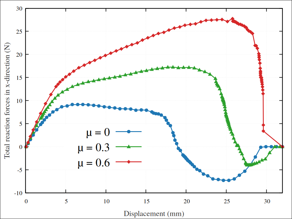
../../_images/RU1_upper.png — Fig. 75 Reaction force in the x-direction, for the upper beam, as function of its displacement for frictionless and frictional cases.#

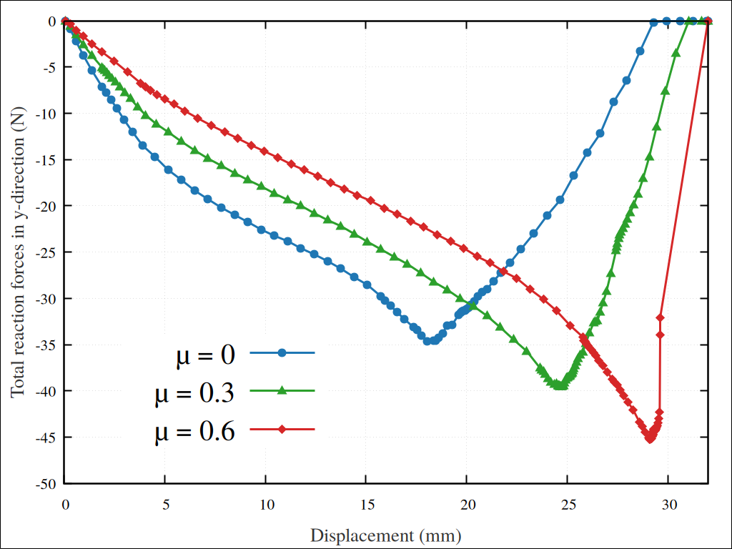
../../_images/RU2_upper.png — Fig. 76 Reaction force in the y-direction, for the upper beam, as function of its displacement for frictionless and frictional cases.#

Downloads

Mesh files

curved_beams.mast
Input files

contact_curved_beams_0_3.inp

Contact between two curved beams

On this page