Elastoplastic analysis of internally pressurised bi-material sphere#

Highlights

Mesh a 3D geometry using Zmaster GUI
Create elsets using functions
Create the material file input using Zair GUI for different elsets
Create the input file using Zair GUI
Launch and visualize the results of a finite element computation
Compute the strain/stress components at the spherical coordinates

Problem specification#

The study proposed in this tutorial focuses on the analysis of a bi-material sphere under internal pressure. This sphere is subjected to a uniform internal pressure of \(P = 100 MPa\). The problem is 1-D axisymmetric in nature, but for demonstration purposes one eighth of the sphere is modelled here and symmetry planes are used.

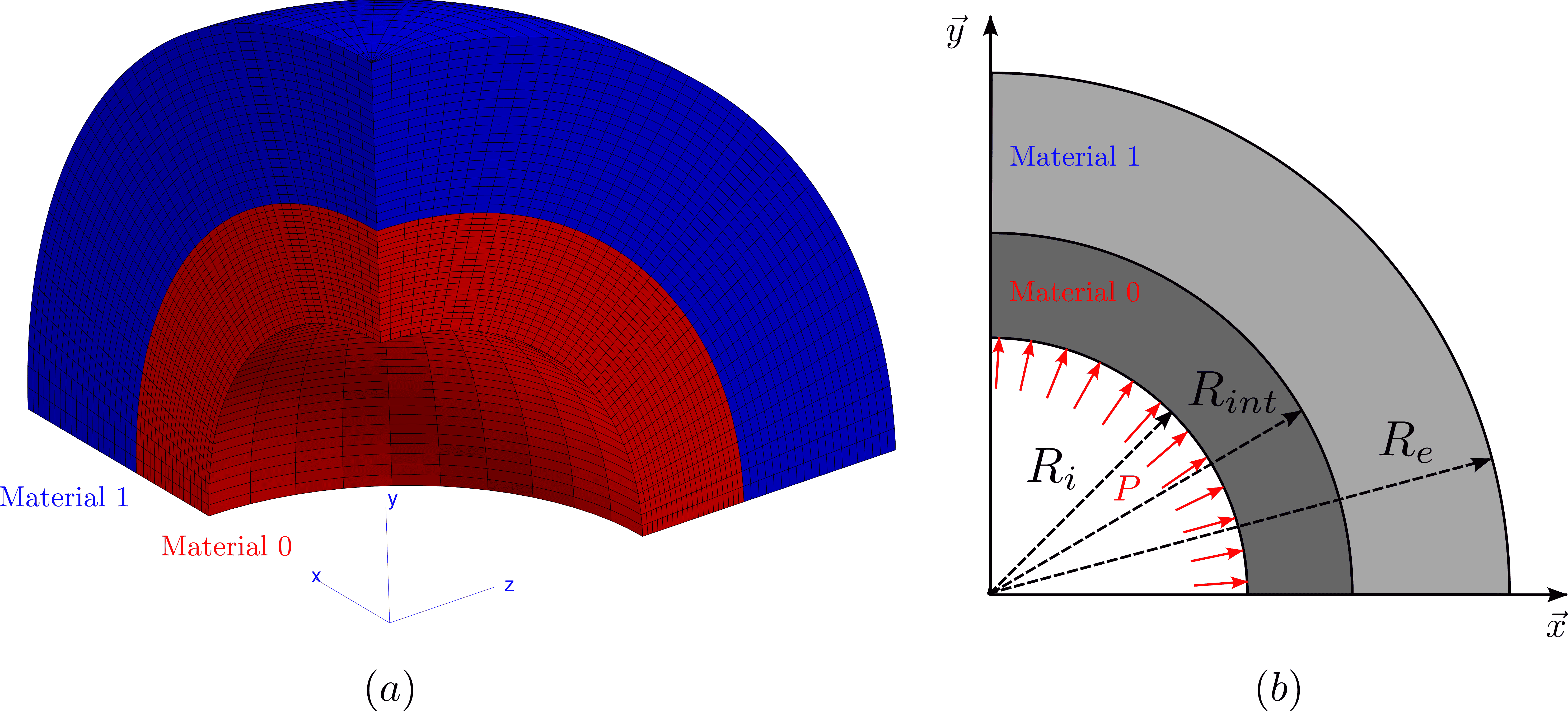
../../_images/model.png — Fig. 42 One eighth of the bi-material sphere (a) sphere’s cross-section (b)#

Table 3 Loading, geometry and material parameters#
Parameters	Numerical value
internal pressure	100 MPa
yield stress \(\sigma_0\)	100 MPa
inner radius \(R_i\)	50 mm
outer radius \(R_e\)	100 mm
interface radius \(R_{int}\) between materials	70mm
material 0
\(~\,~\,\) Young’s modulus	20500 MPa
\(~\,~\,\) Poisson’s coefficient	0.3
\(~\,~\,\) density	\(8.08\times 10^{-9}\) kg.mm\(^{-3}\)
material 1
\(~\,~\,\) Young’s modulus	205000 MPa
\(~\,~\,\) Poisson’s coefficient	0.3
\(~\,~\,\) density	\(8.08\times 10^{-9}\) kg.mm\(^{-3}\)

Analytical solution#

elastic/elastic composite

\[\begin{split}\begin{aligned} \sigma_{rr}^{0}(r)&= \dfrac{a^3 p \left[ A_2 B_2 (b^3 - c^3) \left( A_1 + B_1 \dfrac{b^3}{r^3} \right) + A_1 B_1 (A_2 c^3 + B_2 b^3) \left( 1 - \dfrac{b^3}{r^3} \right) \right]}{A_1 B_1 (A_2 c^3 + B_2 b^3)(b^3 - a^3) + A_2 B_2 (A_1 a^3 + B_1 b^3)(c^3 - b^3)}\\ \sigma_{rr}^{1}(r) &= \dfrac{A_2 B_2 (A_1 + B_1) p a^3 b^3 \left(1 - \dfrac{c^3}{r^3} \right)}{A_1 B_1 (A_2 c^3 + B_2 b^3)(b^3 - a^3) + A_2 B_2 (A_1 a^3 + B_1 b^3)(c^3 - b^3)} \end{aligned}\end{split}\]

\[\begin{split}\begin{aligned} \sigma_{\theta\theta}^{0}(r)&= \sigma_{\phi\phi}^{0}(r)= \dfrac{a^3 p \left[ A_2 B_2 (b^3 - c^3) \left( A_1 - B_1 \dfrac{b^3}{2r^3} \right) + A_1 B_1 (A_2 c^3 + B_2 b^3) \left( 1 + \dfrac{b^3}{2r^3} \right) \right]}{A_1 B_1 (A_2 c^3 + B_2 b^3)(b^3 - a^3) + A_2 B_2 (A_1 a^3 + B_1 b^3)(c^3 - b^3)}\\ \sigma_{\theta\theta}^{1}(r) &=\sigma_{\phi\phi}^{1}(r)= \dfrac{A_2 B_2 (A_1 + B_1) p a^3 b^3 \left(1 + \dfrac{c^3}{2r^3} \right)}{A_1 B_1 (A_2 c^3 + B_2 b^3)(b^3 - a^3) + A_2 B_2 (A_1 a^3 + B_1 b^3)(c^3 - b^3)} \end{aligned}\end{split}\]

where

\[A_1 = \dfrac{\lambda_1(1+\nu_1)}{\nu_1},~ B_1 = \dfrac{2\lambda_1(1-2\nu_1)}{\nu_1},~ A_2 = \dfrac{\lambda_2(1+\nu_2)}{\nu_2},~ B_2 = \dfrac{2\lambda_2(1-2\nu_2)}{\nu_2}\]

Mesh generation#

Geometry creation#

To create the sphere geometry with Zmaster:

Run the command Zmaster sphere.mast in a terminal to open the Zmaster interface. This command will create a file sphere.mast in which the geometry will be stored in text form.
Click on \(\longrightarrow\) to create the points that define the 2d geometry, which in this case is a quarter of a disk.

Enter the coordinates of a point (X, Y, Z), then click GO to create the point. Repeat the process for all points.

#Points      X         Y         Z
       50.       0.        0.
       75.       0.        0.
      100.       0.        0.
       0.       100.       0.
       0.        75.       0.
       0.        50.       0.
       0.        0.        0.

Click on View, Auto-center to view all points.
Click on \(\longrightarrow\) to create the lines connecting points 1 and 2, points 2 and 3, points 4 and 5, and points 5 and 6. Choose 2 points, then click Go. Click on points 1 and 2 to define line 1, which will be created. Next, click on points 2 and 3 to define line 2 and create it. Do the same for to create the other lines.
To create the inner and outer circular arcs, click on \(\longrightarrow\) . In the Create Arc window, select Arc: center, pt1, pt2 to create the arcs using the center and two points, then confirm with OK. Click on the center point no. 7 (0,0,0) then point no. 1 and point no. 6 to create the inner arc. Click on the center point no. 7 (0,0,0) then point no. 2 and point no. 5 to create the arc that separate the two materials. Click on the center point no. 7 (0,0,0) then point no. 3 and point no. 4 to create the outer arc.
Save the progress by clicking on File, Save.

Note

All these steps help to populate the sphere.mast file. If you open it with a text editor, you will notice that there is a section for each created entity (points, lines, arcs).
You can achieve the same result by writing the keywords for each entity and opening it with the command Zmaster sphere.mast to see the result.
You can modify the properties of the created entities directly in the sphere.mast file, for example, it is possible to change the coordinates of the points, the radii of the arcs, etc.

The content of the sphere.mast file:

****master
 ***geometry
  **point point0
   *position 0.000000000000000e+00 0.000000000000000e+00 0.000000000000000e+00
  **point point1
   *position 5.000000000000000e+01 0.000000000000000e+00 0.000000000000000e+00
  **point point2
   *position 7.000000000000000e+01 0.000000000000000e+00 0.000000000000000e+00
  **point point3
   *position 1.000000000000000e+02 0.000000000000000e+00 0.000000000000000e+00
  **point point4
   *position 0.000000000000000e+00 1.000000000000000e+02 0.000000000000000e+00
  **point point5
   *position 0.000000000000000e+00 7.000000000000000e+01 0.000000000000000e+00
  **point point6
   *position 0.000000000000000e+00 5.000000000000000e+01 0.000000000000000e+00
  **line line0
   *p1 point1
   *p2 point2
  **line line1
   *p1 point2
   *p2 point3
  **line line2
   *p1 point4
   *p2 point5
  **line line3
   *p1 point5
   *p2 point6
  **arc arc0
   *p1 point1
   *p2 point6
   *center point0
   *data   5.000000000000000e+01 0.000000000000000e+00 1.570796326794897e+00
  **arc arc1
   *p1 point2
   *p2 point5
   *center point0
   *data   7.000000000000000e+01 0.000000000000000e+00 1.570796326794897e+00
  **arc arc2
   *p1 point3
   *p2 point4
   *center point0
   *data   1.000000000000000e+02 0.000000000000000e+00 1.570796326794897e+00
 ***plotting
  **default_options 1 0 1
****return

Structure meshing#

To mesh the previously created geometry, follow these steps:

If the Zmaster interface is closed, open the geometry file using the command Zmaster sphere.mast.
Start by specifying the desired number of nodes on the geometry boundaries (inner and outer) by clicking on \(\longrightarrow\) , and entering the desired number of nodes for each boundary. Each pair of opposite sides must have the same number of nodes (for example, 20 radially on each line and 40 circumferentially on each arc).
Before meshing the quarter of the disk, you must choose the desired mesh type: structured or free. In this case a structured mesh has been used:
- Click on \(\longrightarrow\) .
- Choose the element group name Elset, element type (cax), linear or quadratic elements Quadratic, normal or reduced integration Normal and, since the mesh contains two linear sides, Sides 2 4 linear.
- Click Start, then select the boundaries in an order such that the lines are numbered 2 and 4 (for example, in this order: 1-inner arc, 2-line #1, 3-outer arc, and 4-line #2) for the two domains \(R0\) and \(R1\) correspond to material_0 and material_1, respectively.
- Click on \(\longrightarrow\) to mesh the geometry.
- Click on to show the mesh.
To create a 3D mesh which is an extend of the planar 2D mesh around the axis y through a sweep rotation.
- Click on \(\longrightarrow\) , then on sweep.
- Enter the angle to sweep through in degrees, num is the number of elements in the extension direction and then confirm with OK.
- Click on \(\longrightarrow\) to mesh the geometry.
- Click on to show the mesh.

Note

All these steps populate the sphere.mast file and create a sphere.geof file, which contains all the nodes and elements of the created mesh.
If you open the sphere.mast file with a text editor, you will notice that additional sections have been added, defining the meshing domain and the type of mesh (structured or free) and the number of nodes in each entity: lines (*cuts 20) and arcs (*cuts 40).
You can obtain the mesh file sphere.geof by adding the previous sections and running the command Zrun -B sphere.mast in a terminal.
You can modify the mesh characteristics in sphere.geof directly from the sphere.mast file; for example, it is possible to change the number of nodes for each entity with (*cuts 20), the type of elements, etc. Then, run the command Zrun -B sphere.mast to create the mesh in the sphere.geof file.

The content of the sphere.geof file:

***geometry
 **node
  70161 3
  1 -1.914284349463475e-14 5.000000000000000e+01 0.000000000000000e+00
  2 9.816846230313904e-01 4.999036202410324e+01 0.000000000000000e+00
  …
 **element
  16000
  1 c3d15 7 6 5 9842 4965 4966 8 4 4964 1 2 3 9843 4963 4962
  2 c3d20 3 9 10 11 12 13 5 4 9843 9845 9844 9842 4963 4967 4968 4969 4970 4971 4965 4964
  3 c3d20 10 14 15 16 17 18 12 11 9845 9847 9846 9844 4968 4972 4973 4974 4975 4976 4970 4969
  …
***group
 **elset R0
  1 2 3 4 5 6 7 8 9 10 11 12 13 14 15 16 17 18 19 20 21
  …
***return

Creation of nsets, bsets, or elsets#

It will be useful to create groups of nodes (nsets), boundary groups (bsets), or element groups (elsets) to apply boundary conditions or to plot stress along a line, for example, to easily apply boundary conditions, boundary groups will be created.

==========  =======================
Bsets       Definition
==========  =======================
inner_wall  x*x+y*y+z*z<50.*50.+0.001
outer_wall  x*x+y*y+z*z>100.*100.-0.001
right       x<0.001
bottom      y<0.001
left        z<0.001
==========  =======================

The steps to define nsets and bsets from bsets :

Click on \(\longrightarrow\) , then on bset. Enter the name of the bset, the function defining the bset, and then confirm with OK.
Repeat this operation for as many bsets as needed.
Click on \(\longrightarrow\) , then save the mesh using File \(\longrightarrow\) Save.

Note

If you open the file sphere.mast with a text editor, you will notice that there are additional sections that have been added, defining the nsets, bsets, or elsets.
If you want to modify this part using a text editor, for example, the function for an bset, simply use the command Zrun -B sphere.mast to create the new nsets and bsets or elsets.

The additional sections in the sphere.mast file:

***mesher
 **sweep
   *elset ALL_ELEMENT
   *prog 1.00000
   *angle 90.0000
   *num 10
   *axis ( 0.00000 1.00000 0.00000 )
   *center ( 0.00000 0.00000 0.00000 )
   *fusion 0.00100000
 **bset
   *type cartesian
   *name inner_wall
   *axes 0 1 2
   *limit 0.00100000
   *func x*x+y*y+z*z<50.*50.+0.001;
   *use_dimension 3
   *req_number -1
 **bset
   *type cartesian
   *name outer_wall
   *axes 0 1 2
   *limit 0.00100000
   *func x*x+y*y+z*z>100.*100.-0.001;
   *use_dimension 3
   *req_number -1
 **bset
   *type cartesian
   *name right
   *axes 0 1 2
   *limit 0.00100000
   *func x<0.001;
   *use_dimension 3
   *req_number -1
 **bset
   *type cartesian
   *name left
   *axes 0 1 2
   *limit 0.00100000
   *func z<0.001;
   *use_dimension 3
   *req_number -1
 **bset
   *type cartesian
   *name bottom
   *axes 0 1 2
   *limit 0.00100000
   *func y<0.001;
   *use_dimension 3
   *req_number -1

In the general case, it is needed to define some particular elsets for the needs of the FE analysis. To define these elsets, it is possible to use function as follows written in a mesher.inp file:

****mesher
 ***mesh sphere.geof
  **open sphere.geof

  **elset mat0         % elset for material 0
   *func x*x+y*y+z*z<70.*70.+0.001;

  **elset mat1         % elset for material 1
   *func x*x+y*y+z*z>70.*70.-0.001;

****return

To launch the mesher use the command Zrun -m mesher.inp, a mesh file named sphere.geof will be replaced. Use the command Zmaster sphere.geof to visualize the new mesh with new elsets.

In order to view nsets, bsets and elsets, click on , a window will open that contain three list :
- the first is for the nsets,
- the second is for the bsets,
- the third is for the elsets.
Select the entity to view and then click on Draw.

Finite element analysis#

Problem definition#

The problem definition, solution method, boundary conditions, and loads are defined in the sphere.inp file using an Auto_reader interface.

Type the command Zmaster sphere.inp in a terminal to create the file where the problem data will be stored.
Click on Options, then Auto reader. A window containing the interface will open.
Click on problem, use Filter selection to search for calcul_mechanical, then select this option and confirm with Set. A tree structure will open below problem, containing all the parameters for defining a mechanical calculation.
Start by defining the mesh that will be used by clicking on mesh_def [...] under mesh, select file, and confirm with Set. Click on file that will appear under mesh_def [...] and enter the name of the mesh file, then validate with Open.
Click on resolution to define the parameters of the solution algorithm. Select void and confirm with Set. A tree structure will appear under void and resolution. Click on sequences [+-], choose sequence, then click on Add and enter the following values for the different parameters under sequence:
- nb sequences => 1
- time => 1.0
- increment => 5
- iteration => 10
- algorithm => p1p2p3 (update tangent stiffness at each iteration)
- ratio:
- type => relative (default): residual divided by the norm of external reaction
- value => 1.e-06
- symmetrize => True
To define the boundary conditions and loads applied to the structure, click on bcs [+-], choose impose_nodal_dof using Filter selection, and confirm with Add. Select the options below to constrain the displacement on the right nset in the vertical direction:
- group (*) => right
- dof (*) => U1
- handler => void => coefficients => 0.0
Select the options below to constrain the displacement on the bottom nset in the vertical direction:
- group (*) => bottom
- dof (*) => U2
- handler => void => coefficients => 0.0
Select the options below to constrain the displacement on the left nset in the horizontal direction:
- group (*) => left
- dof (*) => U3
- handler => void => coefficients => 0.0
To define the loads applied to the structure, click on bcs [+-], and choose pressure.

Select the options below to apply the load on the inner wall nset in the vertical direction:
- group (*) => inner_wall
- handler => void:
- coefficients => -100.0
- tables => tab
Click on table [+-], choose name, and confirm with Add. A tree structure will appear under tables, allowing you to define the evolution of the load over time in the tab table. Select the options below:
- name => tab
- time => 0.0 1.0
- value => 0.0 1.0
Add the previously created material file mat0.mat for the elset mat0 by clicking on groups[+-] and adding a new elset. Click on file_name (*) under file and material, click on ... and select the mat0.mat file, then confirm with Open twice. So the same steps to add the material file mat1.mat for the elset mat1.
Save the problem definition by specifying the file name sphere.inp and clicking the Write button. A sphere.inp file will be created containing the problem data.

The content of the sphere.inp file:

****calcul
 ***table
   **name tab
     *time 0.00000 1.00000
     *value 0.00000 1.00000
 ***mesh
   **file sphere.geof
 ***resolution
   **sequence 1
     *time 1.00000
     *increment 5
     *iteration 10
     *algorithm p1p2p3
     *ratio 1.00000e-06
   **symmetrize
 ***bc
   **pressure
     inner_wall  -100.0000 tab
   **impose_nodal_dof
     right  U1  0.00000
     bottom U2  0.00000
     left   U3  0.00000
 ***material
   **elset mat0
     *file mat0.mat
  **elset mat1
     *file mat1.mat
****return

Material behavior#

To assign an elastic material to elset \(R_0\) of the created mesh, follow these steps:

Click on Options, then Behavior reader. A window opens allowing you to define the material.
Modify the name of the output file by entering something like material1.mat. Choose gen_evp and click on Set. A tree structure will appear on the left side containing the various parameters to define.
Select elasticity from the tree structure, then choose the type of elasticity, for example, isotropic. Then, click on Set. The Young’s modulus and the Poisson’s ratio will be added to the tree structure under isotropic and elasticity.
Click on young(*) to define the Young’s modulus, then choose the application method for the modulus, such as constant, and confirm with Set. Constant will be added below Young. By clicking on constant, the value can be defined.
The Poisson’s ratio is defined in the same way, with a value of 0.3.
To define the material’s density, simply click on the parameter masvol below coefficient, then choose constant, confirm with Set, and finally enter the coefficient value as 8.08000e-09.
Specify the name of the file to something more descriptive, like material0.mat. in the Output file section, then save the material behavior by clicking the Write button. A file named material0.mat will be created in the same folder.

To assign an elastoplastic material with linear isotropic hardening to elset \(R_1\) of the created mesh, follow these steps:

Click on Options, then Behavior reader. A window opens allowing you to define the material.
Modify the name of the output file by entering something like material1.mat. Choose gen_evp and click on Set. A tree structure will appear on the left side containing the various parameters to define.
Select elasticity from the tree structure, then choose the type of elasticity, for example, isotropic. Then, click on Set. The Young’s modulus and the Poisson’s ratio will be added to the tree structure under isotropic and elasticity.
Click on young(*) to define the Young’s modulus, then choose the application method for the modulus, such as constant, and confirm with Set. Constant will be added below Young. By clicking on constant, the value can be defined.
The Poisson’s ratio is defined in the same way, with a value of 0.3.
To define the material’s density, simply click on the parameter masvol below coefficient, then choose constant, confirm with Set, and finally enter the coefficient value as 8.08000e-09.
To achieve elasto-plastic behavior, start by defining the potential by clicking on it, choose gen_evp from the list, and then click on Add. The potential gen_evp will be added to the tree structure.
You need to define the new parameters under gen_evp:
- name => ‘ep’,
- criterion (*) => ‘mises’ and confirm with Set,
- flow (*) => ‘plasticity’ and confirm with Set,
- isotropic => ‘linear’,
- R0 => ‘constant’ => ‘100.0’,
- H => ‘constant’ => ‘2000.0’
Specify the name of the file to something more descriptive, like material1.mat, in the Output file section. Then, save the material behavior by clicking the Write button. A file named material1.mat will be created in the same folder.

Note

All the parameters that have been defined are saved in the files material0.mat and material1.mat.
It is possible to define the material behavior directly without using the interface by entering the keywords and parameter values in this file with a text editor.
You can load a material file in the Behavior_reader interface by clicking on ... to select the file to load, then confirm with Open, and finally click on Load.

The content of the material0.mat file:

***behavior linear_elastic
 **elasticity isotropic
   young  205000.
   poisson  0.300000
 **coefficient
   masvol  8.08000e-09
***return

The content of the material1.mat file:

***behavior gen_evp
 **potential gen_evp ep
  *criterion mises
  *flow plasticity
  *isotropic linear
   R0  100.
   H   2000.
 **elasticity isotropic
   young  205000.
   poisson  0.300000
 **coefficient
   masvol  8.08000e-09
***return

Note

You can plot the stress-strain curve by using the command Zsim material1.mat in a terminal in the same location as the material1.mat file.

Resolution#

Click on , a window will open containing the command Zrun sphere and select Finite element, then click on Go to start the calculation.
It is also possible to start the calculation using a terminal by entering the following command: Zrun sphere.inp.

Post-processing#

Post-processing of results in a spherical local coordinate system:

In order to get stress values in the spherical coordinates, one can use the following post-processing by adding it at the end of the sphere.inp and use the terminal command Zrun -pp sphere.inp to run it:

****post_processing
 ***global_post_processing
  **file integ
  **output_number 1-5
  **process transform_frame
   *local_frame spherical
    (0. 0. 0.)
   *tensor_variables sig
   *tensor_variables eto
****return

Results & discussions#

To display the results:

Click on , a Results window will appear containing displacements (U1, U2), reaction forces (RU1, RU2), which are node results. It also includes stresses (sigmises, sig11, sig22, etc.) and strains (epcum, eto11, eto22, etc.) which are results calculated at Gauss points.
Select the result you wish to display, then click Draw or double-click to display the desired result on the mesh.

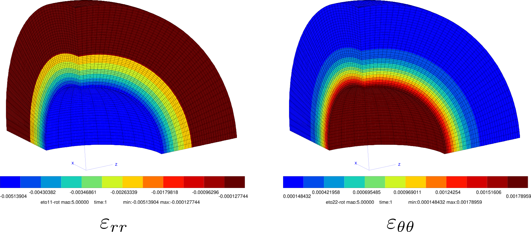
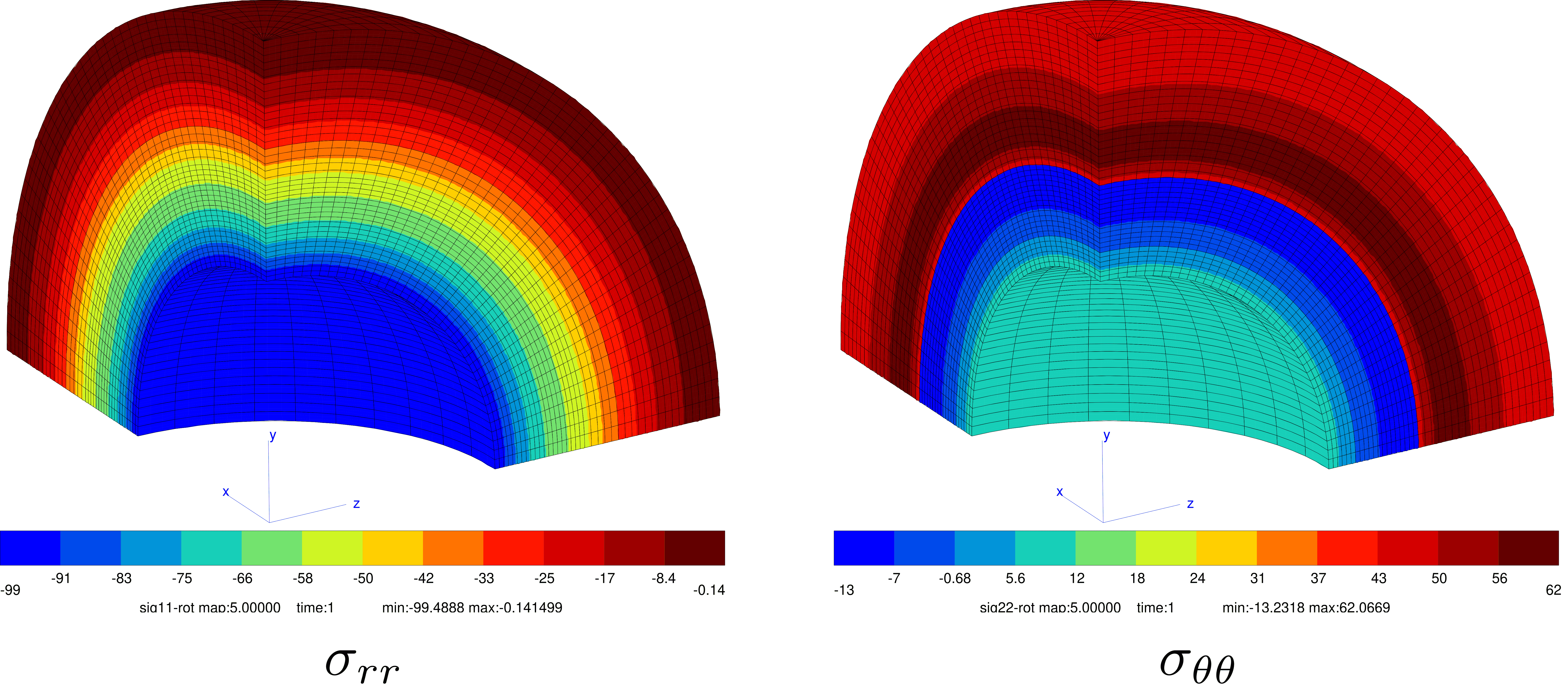
Some examples of calculation results:

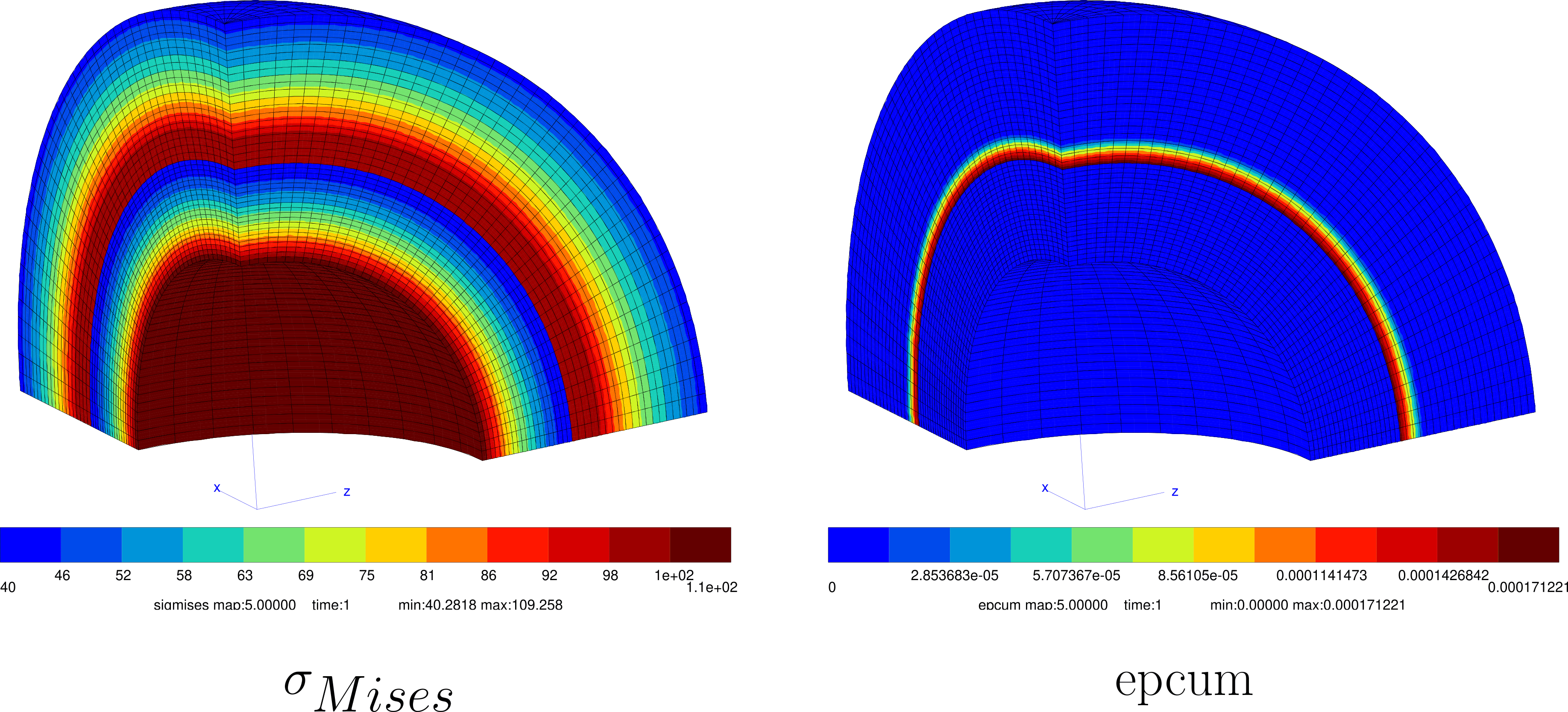
Strain Results:

Stress Results:

Downloads

Mesh files

sphere.mast

mesher.inp
Input files

sphere.inp
Material files

mat0.mat

mat1.mat

Elastoplastic analysis of internally pressurised bi-material sphere

On this page

Elastoplastic analysis of internally pressurised bi-material sphere#

Problem specification#

Analytical solution#

Mesh generation#

Geometry creation#

Structure meshing#

Creation of nsets, bsets, or elsets#

Finite element analysis#

Problem definition#

Material behavior#

Resolution#

Post-processing#

Results & discussions#