Bending

Highlights

• Mesh a 2D/3D plate

• Define boundary conditions to apply a bending.

• Compute the bending moment using post-processing.

Problem specification

Fig. 63 Schematic of a two-dimensional plate subjected to pure bending. For symmetry, only half of the plate will be used in the simulation.

Analytical solution

A foil with a length \(2L\) and width \(2w\) is subjected to pure bending under plane stress conditions and small strains. The applied curvature is denoted by \(\kappa\).

linear elasticity

Consider an isotropic elastic material with Young’s modulus \(E\) and Poisson’s ratio \(\nu\).

• The stress tensor is given by \(\ten{\sigma}=\dfrac{E\kappa x_2}{I_3}\vect{e}_1\otimes\vect{e}_1=\dfrac{-M x_2}{I_3}\vect{e}_1\otimes\vect{e}_1\)

• The strain tensor is given by \(\ten{\varepsilon}=\kappa x_2\left(\vect{e}_1\otimes\vect{e}_1-\nu(\vect{e}_2\otimes\vect{e}_2+\vect{e}_3\otimes\vect{e}_3)\right)\)

• The displacement is given by \(\vect{u}=-\kappa x_1 x_2 \vect{e}_1+\dfrac{\kappa}{2}\left(x_1^2+\nu x_2^2\right)\vect{e}_2\).

where \(I_3=\dfrac{2w^3}{3}\) is the area moment of inertia, and \(M=-EI_3\kappa\) is the bending moment.

elasto-plasticity

The total strain is split in two parts: the elastic strain and the plastic strain

\[\ten \varepsilon = \ten \varepsilon^e+\ten \varepsilon^p\]

Consider a von Mises plasticity model. The yield criterion is given by \(f(\sigma,R)=J_2(\ten \sigma)-\sigma_0-R(p)\) where \(R(p)\) is the isotropic hardening function which depends on the cumulative plastic strain \(p\). At \(y=w\), the stress will reach the yield limit when \(|\sigma_{11}| = \sigma_0\), or when \(|\kappa| = \dfrac{\sigma_0}{E w}\). The width of the elastic zone near the neutral axis is \(2a\) where \(a=\dfrac{\sigma_0}{E|\kappa|}\).

The stress in the elastic/plastic regions is given by

\[\begin{split}\sigma_{11} = \begin{cases} E\kappa x_2, \qquad \text{for } |x_2|\leq a \quad \text{(elastic zone)}\\ \text{sgn}(x_2)\left(\sigma_0+R(p)\right), \qquad \text{for } | x_2 |> a \quad \text{(plastic zone)} \end{cases}\end{split}\]

For a linear isotropic hardening function \(R(p)=H p\), the cumulative plastic strain is given by

\[p(x_2) = \dfrac{\left<E|\kappa x_2|-\sigma_0\right>}{E+H}, \qquad \text{< · > denotes the positive part}\]

The bending moment is given by

\[M = \dfrac{2E\kappa a^3}{3}+ \dfrac{E}{E+H}\left(\sigma_0(w^2-a^2)+\dfrac{2H}{3}\kappa(w^3-a^3)\right)\]

The limit value of the bending moment will be:

• Perfect plasticity (\(H=0\)): \(M_\infty=\sigma_0 w^2\)

• Linear isotropic hardening: \(M_\infty=\dfrac{Ew^2}{E+H}\left(\sigma_0 +\dfrac{2H}{3}\kappa w\right) \xrightarrow{\kappa \to \infty} \infty\)

Mesh generation

Note

To create the mesh, execute

> Zrun -B beam2D.mast

or open beam2D.mast with Zmaster

> Zmaster beam2D.mast

then click on \(\longrightarrow\) .

The following steps will guide you through creating the geometry files from scratch.

2D plate

1. Open Zmaster GUI

2. Click on

3. Create points

   #Points   x     y     z
   
   point0    0.0   -0.5  0.0
   point1    5.0   -0.5  0.0
   point2    5.0   0.5   0.0
   point3    0.0   0.5   0.0
   point4    5.0   0.    0.0
   point5    0.0   0.    0.0
   

   The plate is rectangular and can be meshed using only 4 points. To increase node density near the neutral axis, the plate was subdivided into two rectangles.

4. Create lines

   • Select 2 Points or Segments w/points \(\longrightarrow\) Go.

   • Create the following lines (in any order):

   #Lines   1st point   2nd point
   
   line0    point1      point0
   line1    point3      point3
   line2    point3      point2
   line3    point2      point4
   line4    point4      point1
   line5    point3      point5
   line6    point5      point0
   line7    point5      point4
   

5. Specify the number of nodes at each edge and the progression of nodes for non-uniform nodes’ distribution .

   To refine the mesh at the middle of the plate (neutral axis), set the value of Progression \(>1\), and click near the line node where the mesh should be finer.

   Note that the meaning of the progression value depends on the line definition. If the value of Progression is \(>1\), the spacing between nodes from the first to the last line point decreases; otherwise, it increases.

6. Create Ruled domains

   • Specify the Elset name.

   • Select c2d element type, quadratic, Reduced, and Sides 2 4 linear \(\longrightarrow\) Start.

   • After selecting the bounding edges of each domain, click on Finish.

   • Click on Close.

7. Define boundary sets on which boundary conditions will be applied later

   • left (resp. right) bsets : set Name and select quadratic \(\longrightarrow\) Start, then select the two lines with \(x=0\) (resp. \(x=5\)) in the drawing area \(\longrightarrow\) Finish.

   • left_mid bset: set Name and select Single Point \(\longrightarrow\) Start, then select the point 5 with \(x=y=0\) in the drawing area \(\longrightarrow\) Finish.

8. Mesh the domains

9. Visualize the mesh

3D plate

• To create a 3D geometry, after defining all 2D entities, an extrusion is carried out using a mesher:

  • Click on

  • Scroll down the list and select extension \(\longrightarrow\) New

  • Specify the extension distance and the number of nodes in the extrusion direction num \(\longrightarrow\) OK

• Mesh the domains

Finite element analysis

Finite element formulation

A 2D small strain formulation under plane stress conditions is used:

****calcul
 ***mesh plane_stress
  **file beam2D.geof

Global problem resolution

***resolution
 **sequence           % one loading sequence
  *time 1.            % time range from 0 to 1
  *increment 20       % number of increments. For elastic model use 1
  *ratio 0.1          % convergence ratio set to 0.1%
  *algorithm p1p2p3   % tangent matrix updated for each iteration
 **automatic_time     % automatic time stepping, not needed for elastic model
  *first_dtime 1e-3   % initial time step size
  *divergence 2. 10   % divide time step by 2. if divergence occurs
                      % (max allowed number of divergence is 10)
  *security 1.2       % multiply time step by 1.2 after convergence
                      % if Delta t <= (sequence time/nbr increments)

Boundary conditions

There are various methods to apply bending. Below are two examples:

• a displacement is applied to the right section as \(U_1^{\tt right}=-\theta y\), where math:theta is the rotation angle. The applied curvature is \(\kappa = \theta/L\). For symmetry, the displacement \(U_1 = 0\) is enforced on the left section. To prevent rigid body motion, the displacement \(U_2 = 0\) is imposed on the middle node of the left section.

  ***bc
   **impose_nodal_dof
     right U1 function -0.5*y; time
     left U1 0.
     left_mid U2 0.
  

• The second method involves applying the rotation of the right section as

  ***bc
   **impose_nodal_dof
     left U1 0.
   **linear_rotation right (0. 0.0 1.) (0. 0.5 0.) -20. time;   % apply 20 degrees
  

  Imposing rotation of the right section, will induce boundary effects.

Material behavior

• Elasticity: the material behavior definition is given in elastic.mat file. No integration method is required.

  ***material
    *file elastic.mat
  

  linear_elastic or gen_evp models can be used:

  % elastic.mat file
  ***behavior gen_evp       %   ***behavior linear_elastic
   **elasticity  isotropic  %    **elasticity  isotropic
     young 2e5              %      young 2e5
     poisson 0.3            %      poisson 0.3
  ***return                 %   ***return
  

• Elasto-plasticity: the material behavior definition is given in plastic.mat file. The \(\theta\)-method is used for the integration of constitutive equations.

  ***material
    *file plastic.mat
    *integration theta_method_a 1. 1.e-12 100
  

  % plastic.mat
  ***behavior gen_evp
    **elasticity  isotropic
      young 2e5
      poisson 0.3
    **potential gen_evp ep
     *criterion mises
     *flow plasticity
     *isotropic linear
      R0 100. H 10000.
  ***return
  

Output results

To output nodal values of stress/strain along the liset left over time. In addition, one can specify the variables to output in the results database after **component. To check the available variables, run, for example, Zpreload plastic.mat.

  ***output
  **test results_left.test
   *plot
   *node_extrapolated
   *liset_var left Y sig11 epcum
  **component sig11 eto11 eto22 eto33 eel11 eel22 eel33 epcum
****return   % end of input file

Post-processing

The bending moment around z-axis can be computed using the **process static_torsor. This post-processing computes the torsion moment in terms of the values of nodal reaction forces on left node set:

****post_processing
 ***global_post_processing
  **nset left
  **file node
  **process static_torsor
   *point (0. 0. 0.)
   *file static_torsor.dat    % output file name
****return

The bending moment will be stored in the 10th column of the static_torsor.dat file.

Alternatively, we can use **process torque

****post_processing
 ***global_post_processing
  **file node
  **nset left
  **process torque
   *point (0.,0.5)
   *direction (0.,0.,1.)
****return

The value of bending moment is stored in the 2nd column of problem.post file (the 1st is time).

Results

First, run the finite element problem and the post-processing, and launch Zmaster to visualize the results, using the following commands:

> Zrun bending_plastic
> Zrun -pp bending_plastic
> Zmaster bending_plastic

• To visualize results, click on and choose variables to plot (e.g. epcum) \(\longrightarrow\) Draw

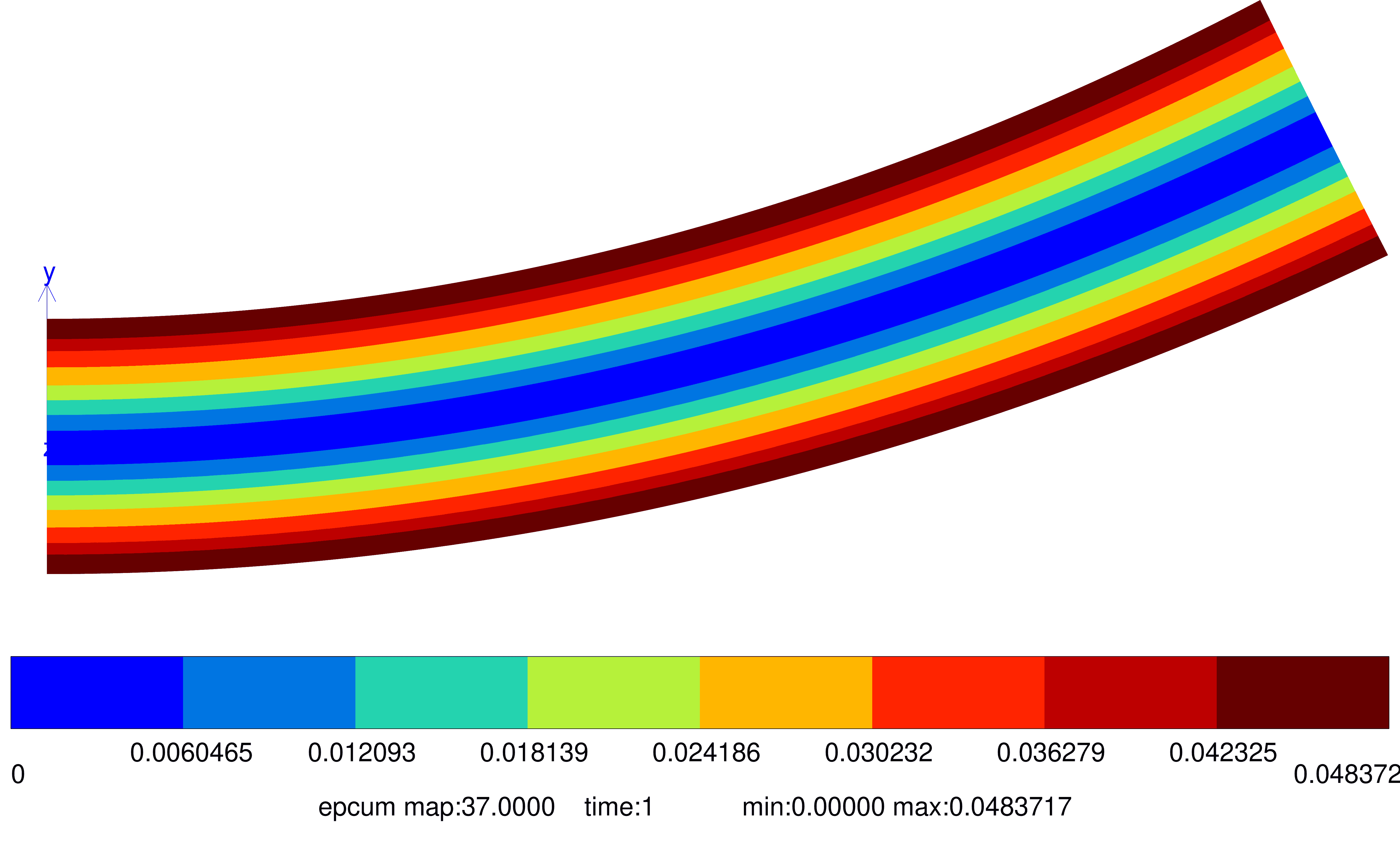
Fig. 64 Cumulative plastic strain

• To plot results along a node set (e.g. left):

  • Click on .

  • Choose the node set left.

  • Choose the maps to plot in Options (e.g. 20, 25, 30). By default, results from the last map are plotted. When ALL is typed in Options text field, all maps are taken into account.

  • Click on More, and uncheck Use deformed coordinates.

  • Export results by specifying the input file name in Curve output, if needed for external processing.

  • To plot results, click on Draw.

  

  Fig. 65 Illustration of how to plot a variable along a node set for different maps.

  

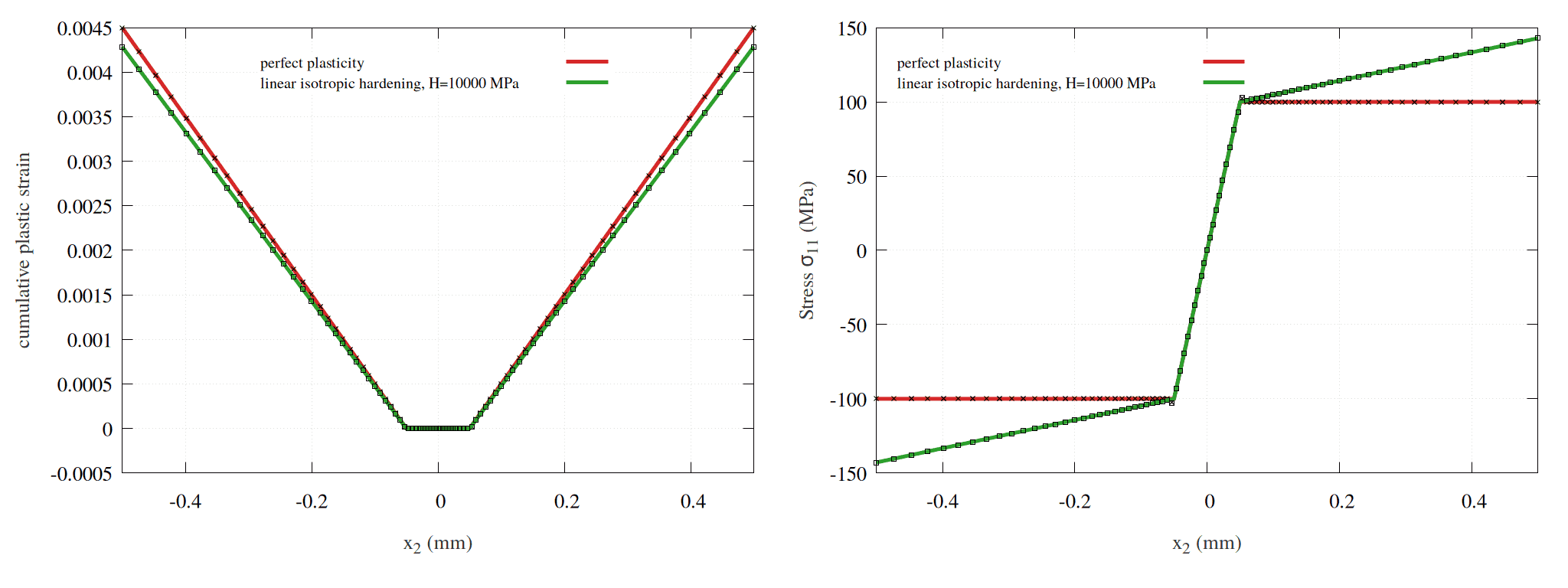
  Fig. 66 The stress and cumulative plastic strain along \(x_2\) for \(\kappa = 0.01\). The solid lines represent the analytical solutions, while the marked dots correspond to FEM results. Note that FEM stress/strain values are extrapolated to nodes.

• The bending moment is obtained after running the post-processing. Next, plot the results using Zmaster or your preferred visualization tool. For plotting with Zmaster, refer to the example.

  

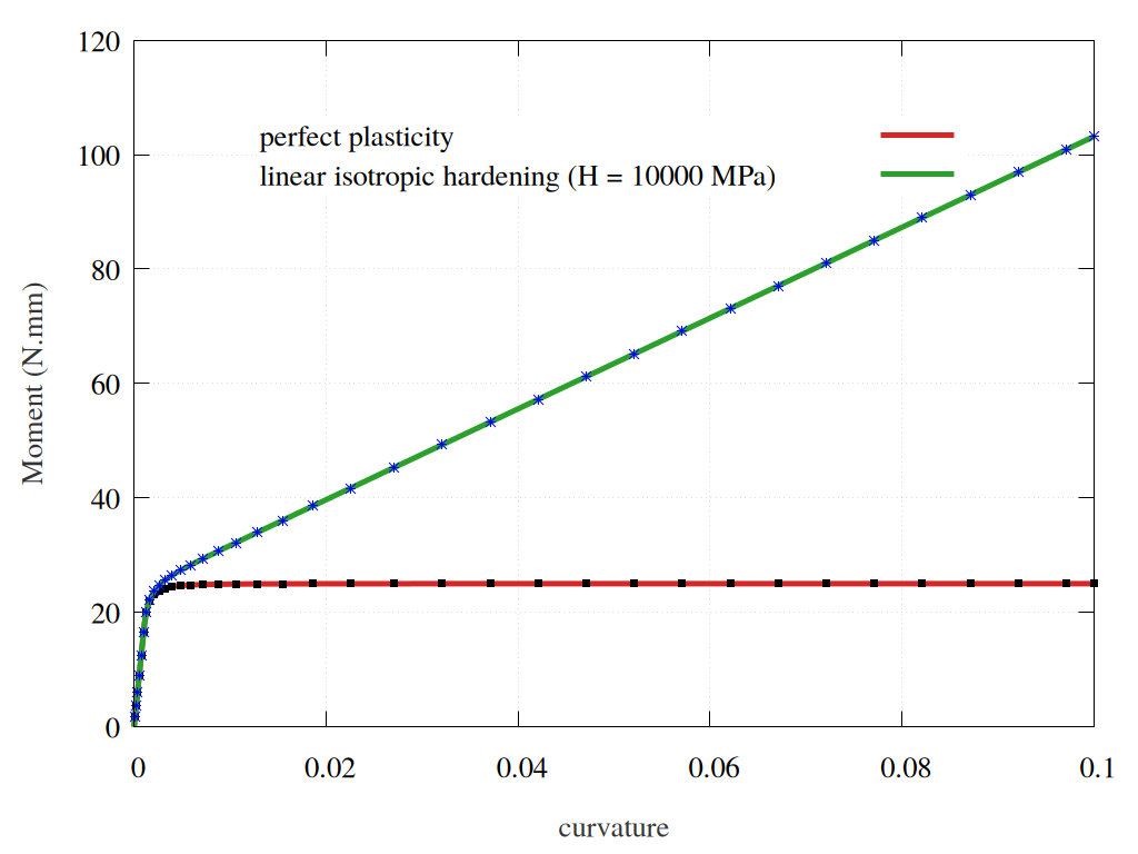
  Fig. 67 Bending moment as a function of curvature for a perfect plastic model and a plastic model with isotropic hardening. The solid lines represent the analytical solutions, while the marked dots correspond to FEM results.

Downloads

• Mesh files

  beam2D.mast

  beam3D.mast

• Input files

  bending_elastic.inp

  bending_plastic.inp

  bending_plastic3d.inp

• Material files

  elastic.mat

  plastic.mat