Torsion of bars (elastoplaticity)#

Highlights

This tutorial explores the following topics:

mesh of a 3D geometry (cylinder) using Zmaster interface GUI and meshers
apply the rotation of node set
compute the torsion moment

Problem specification#

In this tutorial, we will study the evolution of plasticity in a cylindrical bar. First, we will study an elastic bar. Then, an elastoplastic bar with perfect and hardening plasticity will be considered.

../../_images/problem_spec.svg — Fig. 57 (a) torsion of a cylinder with height \(l\) and radius \(R\) (b) cylindrical coordinate frame (c) elastic/plastic regions after yield.#

Analytical solutions#

Isotropic elasticity#

Displacement, strain, and stress fields in the case of small strain isotropic elasticity are given by

\[\begin{split}\begin{aligned} \vect u(r)&=\alpha z r \vect e_\theta \\ \ten \varepsilon (r)&= \dfrac{\alpha}{2} r \left(\vect e_\theta\otimes\vect e_z+\vect e_z\otimes \vect e_\theta\right) \\ \ten \sigma (r)&= \mu \alpha r \left(\vect e_\theta\otimes\vect e_z+\vect e_z\otimes \vect e_\theta\right) \end{aligned}\end{split}\]

where \(\mu=\dfrac{E}{2(1+\nu)}\) is the shear modulus, and \(\alpha\) is the applied rotation angle per length. The applied torque moment is given by

\[\vect{\mathcal{C}}=\int_S \vect{OM}\wedge \left(\ten \sigma\cdot\vect e_z\right) dS = \dfrac{\pi}{2}\mu\alpha R^4\vect e_z\]

Elastoplaticity#

The total strain is split in two parts: the elastic strain related to the stress through the Hooke’s law and the plastic strain

\[\ten \varepsilon = \ten \varepsilon^e+\ten \varepsilon^p\]

Consider a von Mises plasticity model. The yield functions for perfect plasticity, isotropic hardening, and kinematic hardening models are expressed as:

\[\begin{split}\begin{aligned} f(\ten \sigma)=J_2(\ten \sigma)-\sigma_0 & \qquad \text{perfect plasticity} \\ f(\ten \sigma,R)=J_2(\ten \sigma)-\sigma_0-R(p) & \qquad \text{isotropic hardening} \\ f(\ten \sigma,\ten X)=J_2(\ten \sigma-\ten X)-\sigma_0& \qquad \text{kinematic hardening} \end{aligned}\end{split}\]

For the sake of simplicity, we consider linear hardening models, with back stress \(\ten X=\dfrac{2C}{3}\ten \varepsilon^p\), and \(R(p)=H p\) (where \(p\) denotes the cumulative plastic strain).

The applied loading consists of a positive rotation followed by unloading in the reverse direction.

The plasticity occurs when \(J_2(\ten \sigma)=\sigma_0\), where \(J_2(\ten \sigma)=\sqrt{3}\sigma_{\theta z}\) is the von Mises invariant, and \(\sigma_0\) is the yield stress. The plasticity will first appear at \(r=R\) where the value of \(\sigma_{\theta z}\) is at its maximum. Then, the rotation angle per length \(\alpha_{yield}\), and the torque \(\mathcal{C}_{yield}\) that can be applied before yield are:

\[\alpha_{yield}=\dfrac{\sigma_0}{\sqrt{3}\mu R}, \qquad \mathcal{C}_{yield} = \dfrac{\pi R^3 \sigma_0}{2\sqrt{3}}\]

The radius of the elastic zone is given by \(a=\dfrac{\sigma_0}{\sqrt{3}\mu\alpha}\)

The stress \(\sigma_{\theta z}\) is given by

\[\begin{split}\sigma_{\theta z} = \begin{cases} \alpha\mu r, \qquad \text{for } r\leq a \quad \text{(elastic zone)}\\ \dfrac{\sigma_0+\mathcal{H}(p)}{\sqrt{3}}, \qquad \text{for } r>a \quad \text{(plastic zone)} \end{cases}\end{split}\]

where \(\mathcal{H}(p)\) is the hardening function (isotropic or kinematic).

The cumulative plastic strain is given by

perfect plasticity: \(p=\dfrac{\alpha}{\sqrt{3}}(r-a)\)
linear isotropic hardening: \(p=\dfrac{\sqrt{3}\alpha (r-a)}{3+H/\mu}\)
linear kinematic hardening: \(p=\dfrac{\sqrt{3}\alpha (r-a)}{3+C/\mu}\)

The torque, taking into account stresses in both elastic and plastic zones, is given by

\[\mathcal{C}=\dfrac{\pi}{2}\mu\alpha a^4 + 2\pi \int_a^R \sigma_{\theta z} r^2 dr\]

The limit value of the torque (when plasticity reaches the axis) is given by

Perfect plasticity

\[\mathcal{C}_\infty = 2\pi R^3\dfrac{\sigma_0}{3\sqrt{3}}\]
Linear isotropic/kinematic hardening: the torque has no limit due to stress continuously increasing with plastic strain.

Unloading

Now, we consider the case of unloading (the rotation angle \(\alpha_2=\alpha_1-\alpha\) will applied in the opposite direction). The stress in elastic and plastic regions is given by

\[\begin{split}\sigma_{\theta z}(r) = \begin{cases} \alpha \mu r &\qquad \text{for } 0\leq r\leq a~~ ( \text{elastic zone})\\ \dfrac{\sigma_0+\mathcal{H}(p_1)}{\sqrt{3}}- \mu \alpha_2 r & \qquad \text{for } a\leq r\leq R ~~ (\text{plastic zone}) \end{cases}\end{split}\]

The unloading will be elastic until a value of \(\alpha^u_{yield}\) is applied. The yield will appear at \(r=R\), and

perfect plasticity: \(\alpha^u_{yield}=\dfrac{2\sigma_0}{\sqrt{3}\mu R}\),
isotropic hardening: \(\alpha^u_{yield}=\dfrac{2(\sigma_0+Hp_1)}{\sqrt{3}\mu R}\), with \(p_1\) is the cumulative plastic strain before unloading.
linear kinematic hardening: \(\alpha^u_{yield}=\dfrac{2\sigma_0}{\sqrt{3}\mu R}\)

When \(\alpha_2=\alpha_1\), the residual stresses are expressed as

\[\begin{split}\sigma_{\theta z}(r) = \begin{cases} 0 &\qquad \text{for } 0\leq r\leq a\\ \dfrac{\sigma_0+\mathcal{H}(p_1)}{\sqrt{3}}- \mu \alpha_2 r & \qquad \text{for } a\leq r\leq b\\ \dfrac{\sigma_0+\mathcal{H}(p)}{\sqrt{3}} & \qquad \text{for } b\leq r\leq R \end{cases}\end{split}\]

where \(b=\dfrac{2\sigma_0}{\sqrt{3}\mu\alpha_2}\). The cumulative plastic strain in the region \(b\leq r\leq R\) can be written as

perfect plasticity: \(p(r)=p_1(r)+\dfrac{\alpha r}{\sqrt{3}}-\dfrac{2\sigma_0}{3\mu}\)
isotropic hardening: \(p(r)=p_1(r)+\dfrac{\sqrt{3}\mu\alpha r - (2\sigma_0+Hp_1)}{3\mu+\sqrt{3}H}\)
linear kinematic hardening: \(p(r)=p_1(r)+\dfrac{\sqrt{3}\mu\alpha r - 2\sigma_0}{3\mu+\sqrt{3}C}\)

Mesh generation#

Note

To create the mesh, execute

> Zrun -m mesh_cylinder.inp

The following steps will guide you through creating the geometry files from scratch.

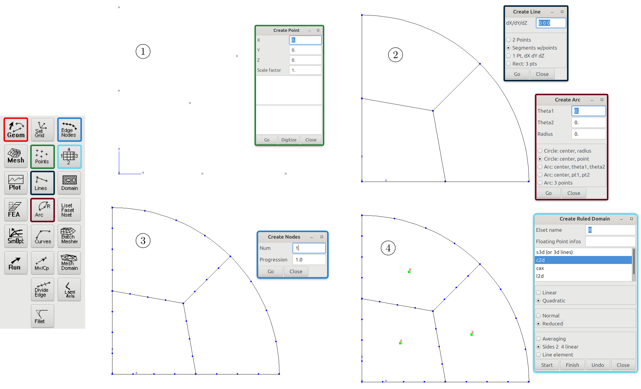
First the mesh of a quarter of a disk is created (disk_quart.mast) using Zmaster interface.

Create points \(\longrightarrow\)

#Points   x        y        z
point0    0.       0.       0.
point1    1.       0.       0.
point2    0.       1.       0.
point3    0.5      0.       0.
point4    0.       5.       0.
point5    0.425    0.425    0.
point6    0.707107 0.707107 0.

Create lines and arcs
Define the number of nodes at each edge
Create ruled domains
Save the project .mast file. (File \(\longrightarrow\) Save)

To obtain the mesh of the cylinder:

Create the mesh of the quarter disk fourth.geof from disk_quart.mast.
Create the symmetrical part of the disk quarter using **symmetry of type line transformer, and use a **union to get the half of a disk.
Create the symmetrical part of the disk half using **symmetry of type line transformer, and use a **union to get the mesh of a full 2D disk.
Extrude the mesh of 2D disk to obtain the mesh of the cylinder. After this operation, the mesh will be made of c3d20r elements. The interpolation is quadratic because the ruled domains (disk_quart.mast) are made of quadratic elements, and the reduced integration is set to *reduced.
Define some useful boundary sets: top, bottom, X. In this case, it is very convenient to use simple functions. For example, the faset top is defined as the faces that has a coordinate z>1.999. The liset X will be used to plot some quantities along the x-axis.

Hint

The command ***shell is used here in order to clean up intermediate meshes ( fourth.geof, half.geof, planar.geof, and disk_quart.geof).
After ***shell, ensure the commands are compatible with the operating system (e.g. rm for Linux, and del for Windows.

% mesh_cylinder.inp file
****mesher
 ***mesh fourth.geof
  **open_mast disk_quart.mast

 ***mesh half.geof
  **open fourth.geof
  **symmetry
   *type line
   *normal (-1. 0. 0.)
  **union
   *add fourth.geof
 ***mesh planar
  **open half.geof
  **symmetry
   *type line
   *normal (0. -1. -1)
  **union
   *add half.geof
 ***mesh cylinder.geof
  **open planar.geof
  **extension
   *reduced
   *distance 2.
   *num 5

  **bset top
   *function z>1.999;
  **bset bottom
   *function z<0.001;
  **bset X *function (z>1.999)*(abs(y)<0.0001)*(x>-0.001); *use_dimension 1
 ***shell rm fourth.geof half.geof planar.geof disk_quart.geof
****return

Finite element analysis#

Finite element formulation#

A small strain formulation is used as

****calcul
 ***mesh  small_deformation
  **file cylinder.geof

Global problem resolution#

***resolution                % by default, Newton methods
 **sequence 4                % 4 loading sequences
  *time  0.15 1. 1.3 2.      % time from 0. to 2.
  *increment 10              % number of increments/sequence, for elastic models use 1
  *iteration 20              % the maximum number of iterations per increment
  *ratio 0.01                % the convergence ratio
  *algorithm p1p2p3          % use Newton-Raphson algorithm
 **automatic_time            % setup the automatic time
  *security 1.2              % increase time step by 1.2 in case of convergence
  *divergence 2. 10          % decrease time step by 2 in case of divergence
                             % maximum number of divergences is 10
  *first_dtime 1e-3          % first time step

Boundary conditions#

***bc                                 % boundary conditions
 **impose_nodal_dof                   % impose nodal degrees of freedom on node sets
   bottom U3 0.                       % set U3=0 on the node set "bottom"
   bottom U2 0.                       % set U2=0 on the node set "bottom"
   bottom U1 0.                       % set U1=0 on the node set "bottom"
 **linear_rotation                    % apply a linear rotation
   top  (0. 0. 1.) (0.,0.,2.)  2. tab % rotate the node set "top" around z-axis,
                                      % where the rotation center is (0,0,1),
                                      % by rotation = 2 degrees * tab
                                      % On "top" nset.

where the table tab is defined as

***table
 **name  tab
  *time  0. 1. 2.
  *value 0. 1. 0.

Note

linear_rotation boundary condition is a linearized version of the **rotation, and should be used with small strain problems.

Material behavior#

***material                                  % set the material model
   *file mat_behavior                        % 'mat_behavior' should be replaced by the right file
   *integration theta_method_a 1. 1.e-10 50  % choose the integration method for
                                             % constitutive equations

Isotropic elasticity#

 % elastic_behavior file
 ***behavior gen_evp
  **elasticity isotropic
    young 200000.
    poisson 0.3
***return

Elastoplasticity#

 % elastoplastic_behavior file
 ***behavior gen_evp
  **elasticity isotropic
    young 200000.
    poisson 0.3
  **potential gen_evp ep
   *flow plasticity
   *criterion mises
   *isotropic linear
    R0 300. H 0.
***return

Post-processing#

To compute stress values in the cylindrical coordinates frame

***global_post_processing
 **file node
 **nset ALL
 **process transform_frame
  *local_frame cylindrical (0. 0. 0.) (0. 0. 1.)
  *tensor_variables sig
  *tensor_size 6

To compute the torque value, the static_torsor post_processing can be used:

***global_post_processing
 **nset top
 **file node
 **process static_torsor
  *point (0. 0. 0.)
  *file static_torsor.dat    % the output result is stored in this file

The torque will be stored in the 10th column of the static_torsor.dat file.

The torque post_processing can also be used:

***global_post_processing
 **file node
 **nset top
 **process torque
  *point (0.,0., 2.)
  *direction (0.,0.,1.)

In this case, torque will be stored in the second column of .post file.

Results#

Small strain elasticity#

First, run the finite element problem and the post-processing, and launch Zmaster to visualize the results, using the following commands:

> Zrun torsion_hpp_elastic
> Zrun -pp torsion_hpp_elastic
> Zmaster torsion_hpp_elastic

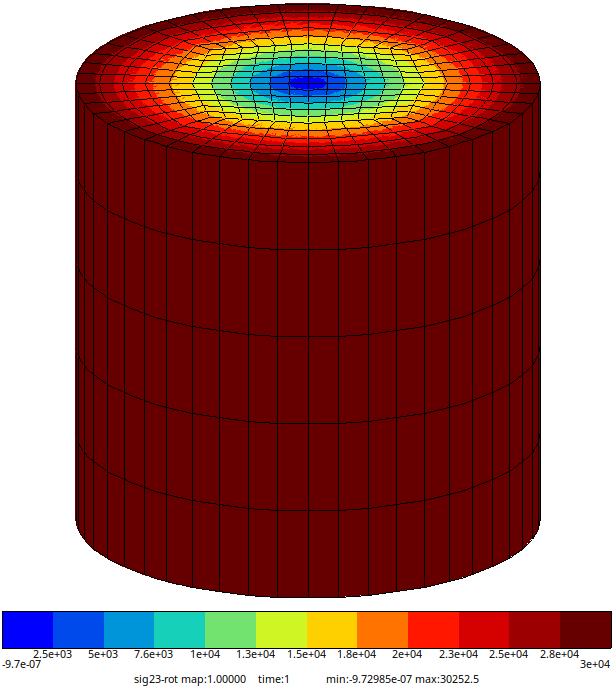
../../_images/sigma_ztheta.png — Fig. 58 Finite element solution: \(\sigma_{\theta z}\) stress (at nodes) for \(E=2\times 10^5\) MPa, \(\nu=0.3\), and \(\alpha=45^\circ/2 mm\).#

Small strain elasto-plasticity#

For brevity, we consider a perfect plastic model with \(\sigma_0=300\) MPa. The same analysis applies to isotropic/kinematic hardening by modifying the material behavior in torsion_hpp_plastic.inp.

Run the following commands:

> Zrun torsion_hpp_plastic
> Zrun -pp torsion_hpp_plastic
> Zmaster torsion_hpp_plastic

To plot the evolution of cumulative plastic strain on one of the outer perimeter nodes:

click on ,
click on Add/Del..,
select node_vals \(\longrightarrow\) New,
set nodes to the node number (e.g. 6577 with \(x=1mm,~y=0mm,~z=2mm\)) \(\longrightarrow\) OK. Now a line node: 6577 is added below liset: … in the plot panel,
Select node: 6577, and choose variables time vs. epcum \(\longrightarrow\) Draw

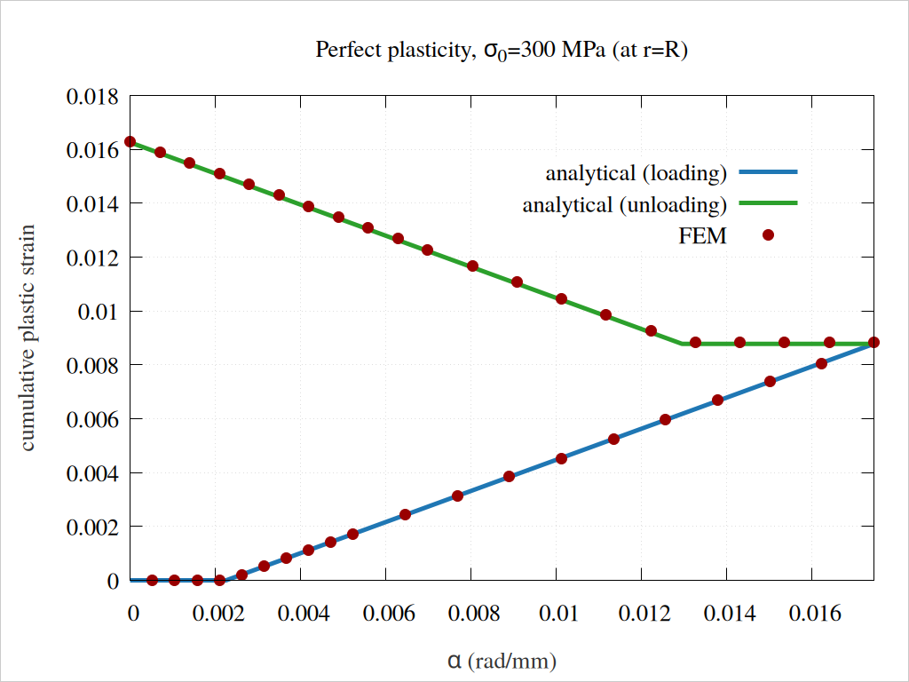
../../_images/epcum_vs_time6577.png — Fig. 59 The cumulative plastic strain in terms of rotation angle per length \(\alpha\).#

To visualize stress click on , select sig23-rot (i.e. \(\sigma_{\theta z}\)). The last results map depicts the residual stress after complete unloading.

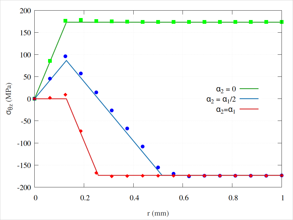
../../_images/residual_stress.png — Fig. 60 The stress \(\sigma_{\theta z}\) after unloading. The solid lines represent the analytical solutions, while the marked dots correspond to FEM results. Note that FEM stress values are extrapolated to nodes.#

The figure Fig. 61 depicts the evolution of the torque in terms of the applied rotation angle \(\alpha\).

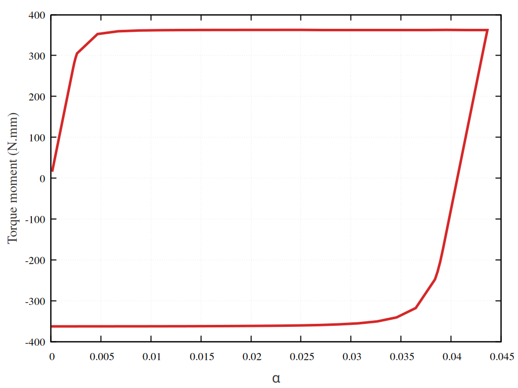
../../_images/torque_vs_alpha.png — Fig. 61 evolution of the torque in terms of the applied rotation angle \(\alpha\).#

Large deformations#

Poynting effect

The Poynting effect is a nonlinear mechanical behavior frequently observed in soft solids, including rubber, gels, and biological tissues. When these materials undergo shear or torsional deformation, they either stretch or compress in the direction perpendicular to the plane of the applied shear or twist.

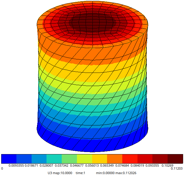
../../_images/U3_rivlin_poynting.png — Fig. 62 The displacement \(U_3\) for an Rivlin hyperelastic model (\(\alpha=0.5\)).#

For a small strain model, the displacement in the \(x_3\)-direction will vanish.

Note

**linear_free_rotation (or **free_rotation for a finite strain model) boundary condition should be used in order to allow displacement in the \(x_3\)-direction.

Downloads

Mesh files

disk_quart.mast

mesh_cylinder.inp
Input files

torsion_hpp_elastic.inp

torsion_hpp_plastic.inp

torsion_incomp.inp
Material files

perfect_plastic.mat

linear_iso_plastic.mat

linear_kine_plastic.mat

Torsion of bars (elastoplaticity)

On this page

Torsion of bars (elastoplaticity)#

Problem specification#

Analytical solutions#

Isotropic elasticity#

Elastoplaticity#

Mesh generation#

Finite element analysis#

Finite element formulation#

Global problem resolution#

Boundary conditions#

Material behavior#

Isotropic elasticity#

Elastoplasticity#

Post-processing#

Results#

Small strain elasticity#

Small strain elasto-plasticity#

Large deformations#